Robust Adversarial Quantification via Conflict-Aware Evidential Deep Learning

Introduction

#

I’ll be presenting our paper “Robust Adversarial Quantification via Conflict-aware Evidential Deep Learning” which is a part of our European project, GuardAI, at ICLR ‘26 in Rio de Janeiro, Brazil. In this blog post, I’ll walk through the work in a more informal way and explain how our method, C-EDL, works. If you’re interested, you can check out the paper beforehand.

At a high level, C-EDL is a lightweight, post-hoc method for improving uncertainty estimation in evidential deep learning models, particularly under distributional shift and adversarial perturbations. Instead of retraining models or introducing heavy computational overhead, C-EDL operates on top of pretrained evidential models by probing how stable their predictions are under small, label-preserving transformations. When the model disagrees with itself, we treat this as a signal of uncertainty and adjust its confidence accordingly.

To keep things accessible, I’ll first give a quick intuition behind uncertainty in deep learning, then walk through how C-EDL works, show some key results, and finish with a few thoughts on where this line of work could go next.

Motivation

#

Deep learning models can be very accurate, but accuracy alone is not enough when a model is deployed in the real world. In high-stakes settings, the real question is not just whether a model gets the right answer on average, but whether it can recognize when its prediction should not be trusted. Inputs may look different from the training data (for example, a pedestrian detection camera may encounter animals too), or they may be deliberately perturbed in subtle ways (i.e., from an adversarial attack), and in both cases an overconfident mistake can be much more harmful than an uncertain one. This is why uncertainty quantification (UQ) matters: we want models that can say not only what they predict, but also how certain they are [1].

One appealing way to do this is through Evidential Deep Learning (EDL) [2]. Many UQ methods estimate uncertainty using computationally heavier machinery, such as ensembles [3], Bayesian approximations [4], or repeated stochastic forward passes [5]. By contrast, EDL stays lightweight: rather than outputting just a single class prediction, it produces evidence for each class and represents its prediction as a Dirichlet distribution. In practice, this means the model can express both its preferred class and how much overall evidence it has collected in support of that decision, all in a single deterministic forward pass. That makes EDL especially attractive when you want efficient uncertainty estimation without the extra cost of repeated sampling or multiple models. I’ve also included an interactive EDL diagram below so you can play around with the idea and build some intuition for how the evidence and uncertainty behave for in-distribution (ID) and out-of-distribution (OOD) data.

But that single forward pass is also where the trouble starts. Since EDL only sees one version of the input at test time, it has no built-in way to check whether its prediction is stable. If an adversarial perturbation nudges the model in the wrong direction, the model can still respond with high confidence, even when it really should not. So while EDL is efficient, it can still be brittle under attack [6]. This is the motivation for our proposed method, C-EDL.

C-EDL

#

C-EDL is designed as a lightweight, post-hoc uncertainty method for evidential classifiers, so it does not require retraining the model or changing its original learning procedure. Instead, it works on top of a pre-trained EDL model, probing how stable the model’s evidential predictions remain under small, label-preserving transformations of the input. The key idea is simple: if those predictions remain consistent, the model can keep its original confidence, but if they disagree, that disagreement should be treated as a sign of uncertainty. The method therefore has two main steps: first, it generates a set of transformed views and collects the corresponding evidence, and second, it measures conflict across those views and adjusts the final prediction accordingly. A high-level overview is shown in the figure below.

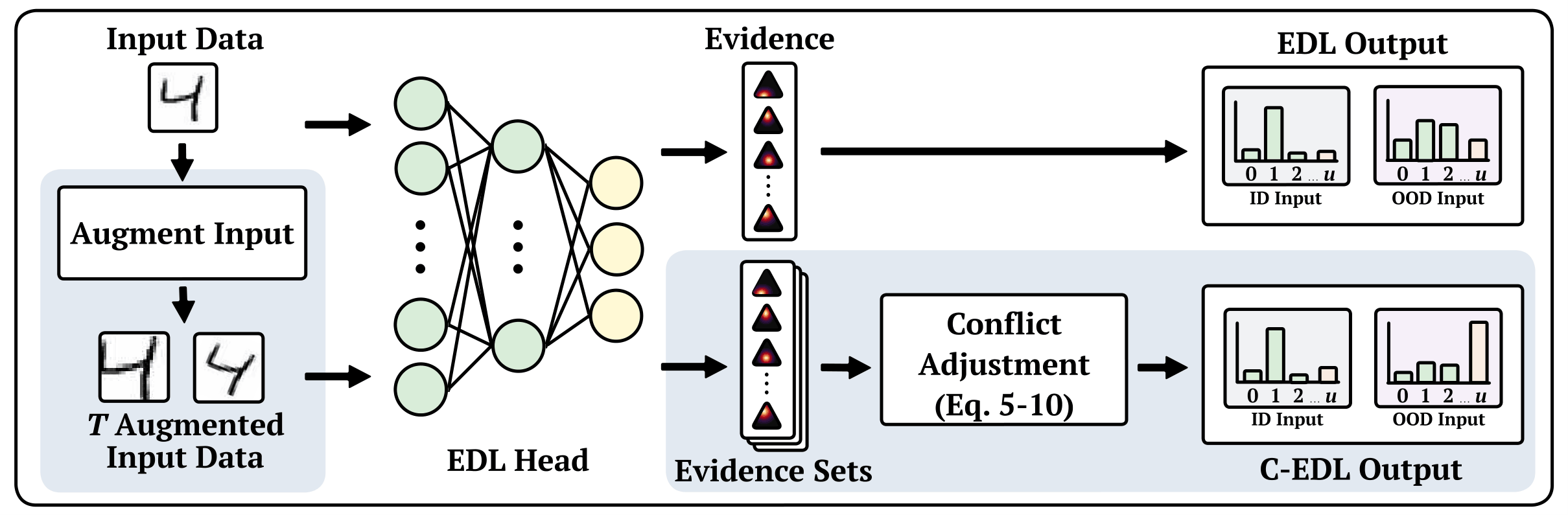
Formally, for an input \( x \), C-EDL applies a set of \( T \) label-preserving metamorphic transformations \( { \tau_1, \dots, \tau_T } \), chosen so that the true label should not change, i.e. \( f^’(\tau_t(x)) = f^’(x) \) for all \( t \in {1, \dots, T} \). Each transformed input \( \tau_t(x) \) is then passed independently through the pre-trained EDL model, producing a Dirichlet parameter vector \( \alpha^{(t)} = (\alpha_1^{(t)}, \dots, \alpha_K^{(t)}) \). This gives a set of evidential outputs \( A = { \alpha^{(1)}, \alpha^{(2)}, \dots, \alpha^{(T)} } \). The intuition is that a robust model should produce similar evidence across all of these views. If the evidence changes a lot, then the model is revealing that its belief is fragile.

C-EDL then quantifies this fragility through two complementary forms of conflict. The first is intra-class conflict, which measures how much the evidence for each class varies across the transformed views. This is defined as:

\( C_{\mathrm{intra}} = \frac{1}{K}\sum_{k=1}^{K} \frac{\sigma({\alpha_k^{(t)}}_{t=1}^{T})}{\mu( {\alpha_k^{(t)}} _{t=1}^{T} ) + \epsilon} \)

def calculate_cintra(self, evidence):
    evidence = np.asarray(evidence)
    epsilon = 1e-8
    std_dev = np.std(evidence, axis=2)
    mean_evidence = np.mean(evidence, axis=2)
    normalized_std = std_dev / (mean_evidence + epsilon)
    return np.mean(normalized_std, axis=1)

where \( \sigma(\cdot) \) and \( \mu(\cdot) \) denote the standard deviation and mean, and \( \epsilon > 0 \) is a small constant for numerical stability. If a class receives very inconsistent evidence across transformations, then \( C_{\mathrm{intra}} \) increases.

The second is inter-class conflict, which captures competition between classes within each transformed prediction. Intuitively, this becomes large when two or more classes are simultaneously supported with similar, non-trivial evidence. In the paper, this is defined as:

\( C_{\mathrm{inter}} = \frac{1}{T}\sum_{t=1}^{T} \left( 1 - \exp\left( -\beta \sum_{k=1}^{K}\sum_{j=k+1}^{K} \frac{\min(\alpha_k^{(t)}, \alpha_j^{(t)})}{\max(\alpha_k^{(t)}, \alpha_j^{(t)})} \cdot \frac{\min(\alpha_k^{(t)}, \alpha_j^{(t)})}{\sum_{k=1}^{K}\alpha_k^{(t)}} \cdot 2 \right)^2 \right) \)

def calculate_crun_inter(self, evidence, beta):
    B, C, R = evidence.shape
    i_idx, j_idx = np.triu_indices(C, k=1)
    krun_inter_values = np.zeros(B)
    for b in range(B):
        e = evidence[b]
        denom_sum = np.sum(e, axis=0)
        ei = e[i_idx]
        ej = e[j_idx]
        min_e = np.minimum(ei, ej)
        max_e = np.maximum(ei, ej)
        valid = max_e > 0
        min_e_valid = np.where(valid, min_e, 0)
        max_e_valid = np.where(valid, max_e, 1)
        denom_sum_safe = np.where(denom_sum == 0, 1, denom_sum)
        conflict = (min_e_valid / max_e_valid) * (min_e_valid / denom_sum_safe) * 2
        sum_squared = np.sum(conflict ** 2, axis=0)
        mean_sum_power = np.sqrt(sum_squared)
        krun_inter_values[b] = np.mean(1 - np.exp(-beta * mean_sum_power))
    return krun_inter_values

where \( \beta > 0 \) controls how sharply contradiction is penalised. The key idea is simply that \( C_{\mathrm{inter}} \) rises when the model is torn between competing classes rather than confidently favouring one.

These two scores are then combined into a single total conflict value:

\( C = C_{\mathrm{inter}} + C_{\mathrm{intra}} - C_{\mathrm{inter}}C_{\mathrm{intra}} - \lambda(C_{\mathrm{inter}} - C_{\mathrm{intra}})^2 \)

def compute_c_total(self, c_inter, c_intra):
    lambda_penalty = 0.5
    penalty_grid = lambda_penalty * (c_inter - c_intra)**2
    c_total = c_inter + c_intra - c_inter * c_intra - penalty_grid
    return np.clip(c_total, 0, 1)

where \( \lambda \in [0,1] \) controls how much to penalize asymmetric disagreement between the two types of conflict. Once this total conflict is computed, the transformed evidential outputs are first averaged, \( \bar{\alpha}_k = \frac{1}{T}\sum _{t=1}^{T} \alpha_k^{(t)} \), and then adjusted using an exponential decay, \( \tilde{\alpha}_k = \bar{\alpha}_k \exp(-\delta C) \), where \( \delta > 0 \) controls how aggressively conflict reduces the evidence. This is the main correction step in C-EDL: if conflict is low, then the evidence stays close to the original value, but if conflict is high, the total evidence is reduced. In the interactive example, this is exactly what can be observed when changing \( \delta \): larger values make the adjusted evidence shrink more quickly, which in turn increases uncertainty.

Finally, the usual EDL quantities are recomputed using the adjusted Dirichlet parameters. The adjusted Dirichlet strength is \( \tilde{S} = \sum_{k=1}^{K}\tilde{\alpha}_k \), and the resulting uncertainty mass is \( \tilde{u} = \frac{K}{\tilde{S}} \). So the overall effect is straightforward: higher conflict leads to lower total evidence, which leads to higher uncertainty. For ID inputs, the transformed views tend to agree, so the conflict remains small and C-EDL stays close to the original EDL prediction. For OOD or adversarial inputs, disagreement tends to grow, so C-EDL suppresses the evidence and produces a more cautious uncertainty estimate. That is the core mechanism behind the method, and the interactive pipeline below lets you explore exactly how the parameters and intermediate values contribute to that final behaviour.

Results

#

I do not want to overload this post with too many tables and figures, so I will just highlight the main results here and leave the full set of experiments to the paper.

We evaluate C-EDL across a range of in-distribution, out-of-distribution, and adversarial settings, comparing it against several competitive uncertainty quantification baselines. Alongside the main C-EDL method, which uses metamorphic transformations to generate multiple task-preserving views of each input, we also evaluate an MC variant that instead uses Monte Carlo Dropout. This helps show that the improvements are not simply due to having multiple predictions, but to the structured transformations and conflict-aware adjustment used by C-EDL. We also include an EDL++ variant, which averages evidence across views but does not apply conflict adjustment, allowing us to isolate the contribution of that step.

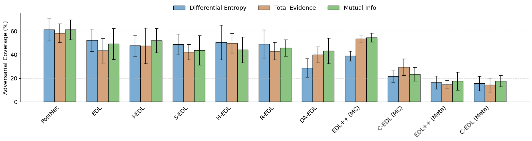
To study adversarial robustness, we evaluate all methods under three attacks, L2PGD, FGSM, and Salt-and-Pepper noise, while varying the perturbation strength \( \epsilon \). We also compare three ID-OOD threshold metrics: differential entropy, total evidence, and mutual information. You can see these in the two Figures below.

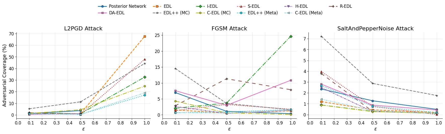
The main trend is clear. As attack strength increases, standard EDL retains far more adversarial inputs, especially under L2PGD, whereas both C-EDL variants remain much lower. This means C-EDL is better at treating attacked inputs as unreliable rather than falsely accepting them as in-distribution.

The comparison between the two C-EDL variants is also important: the metamorphic version generally performs best, showing that the gains are not just from having multiple predictions, but from using structured, label-preserving transformations and then measuring the conflict between them.

The threshold results tell a similar story. Across all three threshold metrics, the C-EDL variants consistently achieve lower adversarial coverage than the baselines, showing that the method is robust to the choice of uncertainty score rather than relying on one specific threshold.

Conclusion

#

In this paper, we introduced C-EDL, a lightweight post-hoc uncertainty quantification approach for evidential deep learning models. By generating multiple label-preserving views of an input, measuring the conflict between the resulting evidential predictions, and reducing evidence when disagreement is high, C-EDL improves the detection of out-of-distribution and adversarial inputs without requiring model retraining. Future work will look at extending the approach beyond classification, reducing the number of required transformations, and exploring how conflict-aware evidential adjustment can be used in other uncertainty-sensitive settings. I encourage you to read the full paper for all of the details and even check out the codebase linked at the bottom of the page.

References

#

[1] Abdar, M., Pourpanah, F., Hussain, S., Rezazadegan, D., Liu, L., Ghavamzadeh, M., Fieguth, P., Cao, X., Khosravi, A., Acharya, U.R. and Makarenkov, V., 2021. A review of uncertainty quantification in deep learning: Techniques, applications and challenges. Information fusion, 76, pp.243-297.

[2] Sensoy, M., Kaplan, L. and Kandemir, M., 2018. Evidential deep learning to quantify classification uncertainty. Advances in neural information processing systems, 31.

[3] Lakshminarayanan, B., Pritzel, A. and Blundell, C., 2017. Simple and scalable predictive uncertainty estimation using deep ensembles. Advances in neural information processing systems, 30.

[4] Goan, E. and Fookes, C., 2020. Bayesian neural networks: An introduction and survey. In Case Studies in Applied Bayesian Data Science: CIRM Jean-Morlet Chair, Fall 2018 (pp. 45-87). Cham: Springer International Publishing.

[5] Gal, Y. and Ghahramani, Z., 2016, June. Dropout as a bayesian approximation: Representing model uncertainty in deep learning. In international conference on machine learning (pp. 1050-1059). PMLR.

[6] Kopetzki, A.K., Charpentier, B., Zügner, D., Giri, S. and Günnemann, S., 2021, July. Evaluating robustness of predictive uncertainty estimation: Are Dirichlet-based models reliable?. In International Conference on Machine Learning (pp. 5707-5718). PMLR.

Codebase

#