
💡 Update
Added Label-Smoothed Cross-Entropy loss to the blog!
Introduction#
Neural networks are often evaluated almost entirely through their outputs. For an image classification problem, we provide an image to a model and measure whether the resulting prediction is correct. However, the prediction itself tells us relatively little about how the model has represented the input space internally.
Between the raw image and the final classification layer, neural networks learn increasingly abstract representations of their inputs. These representations, commonly referred to as embeddings, are fundamental to modern deep learning. Ideally, images which share useful characteristics occupy similar regions of the learned representation space, while sufficiently different inputs become separable.
In this post, I want to help people who are still learning parts of deep learning and answer the question: How does the choice of training objective influence the geometry of the representation learned by a neural network? To investigate this, I train the same architecture on the same dataset using several different loss functions and visualise the resulting embedding spaces throughout training so you can interact with these learnt embedding space and learn for yourself.
What are Embeddings?#
First, it is useful to first understand what an embedding actually is and represents. As an image is input through a neural network, it is gradually transformed from raw pixel values into a numerical representation containing features that are useful for the task the model is trying to solve. Near the end of a classifier, we can think of an image as being represented by a vector:
$$ Z = [z_1, z_2, \ldots, z_d] $$
where \(d\) is the dimensionality of the representation. This vector is what we refer to as an embedding.
Now, in a normal neural network, this embedding could contain hundreds or thousands of dimensions. This gives the model plenty of space to represent useful information for very complex tasks, but it makes the representation difficult for us to directly inspect. Techniques such as PCA, t-SNE and UMAP are often used to project these high-dimensional embeddings into two dimensions for visualisation, although the resulting plot is then a transformed view of the original representation. So for this experiment, and to not teach you based off approximations of embeddings, I instead force the network into a bottleneck near the end and learn an embedding with only two dimensions:
$$ Z = [z_1, z_2] $$
Of course, restricting a neural network to only two embedding dimensions creates a significant information bottleneck and is unlikely to give the best possible classification performance. However, that is not really the aim here. Instead, it gives us a simple way to directly observe how a neural network reorganises its representation space as it learns.
Experimental Setup#
For all experiments in this post, I use the CIFAR-10 image classification dataset as somewhat hard toy dataset. CIFAR-10 contains $32 \times 32$ colour images belonging to ten classes: airplane, automobile, bird, cat, deer, dog, frog, horse, ship and truck.
To keep the comparison between loss functions as controlled as possible, every experiment uses the same small convolutional neural network architecture. The only thing that changes between experiments is the training objective. The model follows the general structure:
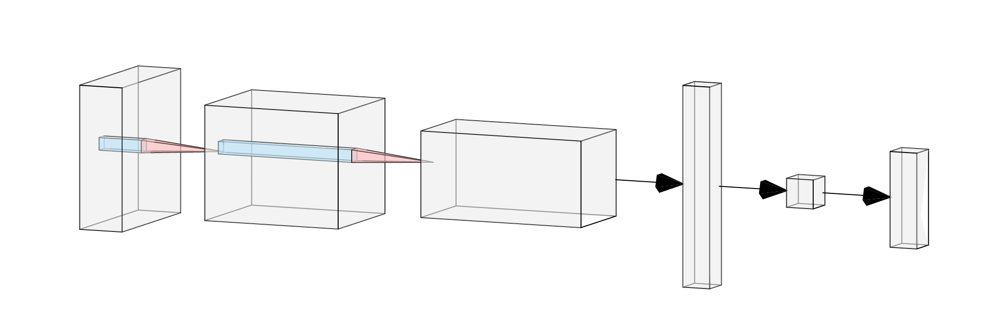
The model takes a 32 × 32 RGB image, passes it through three convolutional blocks with 32, 64, and 128 channels, compresses the resulting features into a 128-dimensional vector, maps this to a 2-dimensional embedding, and finally uses a linear layer to produce 10 CIFAR-10 class logits.

This also gives us another useful property. Because the final classifier operates directly on the two-dimensional embedding, we can visualise not only where the images are placed, but also the decision regions learned by the classifier. In the interactive plots throughout this post, each point represents a CIFAR-10 image, while the coloured background shows which class the model would predict at any position in the embedding space.
Training Objectives#
With the architecture and dataset fixed, the main variable in the following experiments is the training objective. Each objective provides a different signal about what constitutes a good prediction and, consequently, can encourage the network to organise its internal representation in different ways.
For each objective, I visualise how the embedding space evolves throughout training and how the final linear classifier partitions that space. Make sure to mess around with the interactive plots!
Probabilistic Classification Losses#
We begin with objectives that train the network by comparing its predicted class probabilities against a target probability distribution. These losses primarily focus on producing correct and well-calibrated class predictions, rather than directly imposing a particular structure on the embedding space.
Cross-Entropy Loss#
Cross-entropy [1] is the standard objective used for multi-class classification and provides a useful baseline for the comparisons that follow. For a single training example, the loss can be written as:
$$ \mathcal{L}_{CE} = - \sum^{C}_{c=1} y_c \log(p_c) $$
where \(p_c\) is the probability assigned by the model to the correct class. The objective therefore penalises the network when it assigns a low probability to the true class, with increasingly large penalties as that probability approaches zero.
As you can see in the interactive plot above, cross-entropy attempts to organise the embedding space into regions in which images from the same class can be correctly separated by the final classifier. As training progresses, the initially unstructured embeddings begin to move into increasingly class-specific regions, while the decision boundaries adapt alongside them. However, cross-entropy does not explicitly encourage samples from the same class to form compact clusters; it only rewards the model for assigning a higher probability to the correct class. As a result, samples can remain relatively dispersed within their decision region, and some overlap between visually similar classes remains, particularly given the restrictive two-dimensional bottleneck. The model can also continue reducing the loss by moving correctly classified samples further into their respective decision regions, increasing the separation between the correct and competing class logits.
Label-Smoothed Cross-Entropy Loss#
Label smoothing modifies the standard cross-entropy objective by replacing the hard one-hot target distribution with a slightly softened version. Instead of assigning probability 1 to the correct class and 0 to every other class, a small amount of probability mass is distributed across the remaining classes. For \(C\) classes and smoothing parameter \(\epsilon\), the smoothed target can be written as:
$$ \tilde{y}_c = (1-\epsilon)y_c + \frac{\epsilon}{C} $$
The corresponding cross-entropy loss is then:
$$ \mathcal{L}_{CE} = - \sum^{C}_{c=1} \tilde{y}_c \log(p_c) $$
In these experiments, I use \(\epsilon = 0.1\). For CIFAR-10, this means that the target probability for the correct class becomes \(0.91\), while each of the remaining classes receives a target probability of \(0.01\).
The main effect that you can see in the interactive plot is that the network is no longer encouraged to push the probability of the correct class arbitrarily close to 1. This reduces the incentive to produce extremely large differences between the correct and incorrect class logits, which can help limit overconfidence and act as a form of regularisation. You can see this visually as the whole embeddings space has less outliers or clusters spiking outwards. The downside of this regularisation on this experiment is a slightly weaker test accuracy of 59.94% compared to 62.15% for standard cross-entropy.
Conclusion#
The aim of this post was to make representation learning a little more tangible by directly visualising the space a neural network learns during training. By constraining the model to a two-dimensional bottleneck, the embeddings shown throughout the post are not projections produced afterwards, but the actual representations used by the final classifier.
If you would like to explore the implementation, reproduce the experiments, or add additional training objectives, the full codebase is available below.
References#
[1] Goodfellow, I., Bengio, Y., Courville, A. and Bengio, Y., 2016. Deep learning (Vol. 1, No. 2, pp. 1-800). Cambridge: MIT press.