
Introduction#
Uncertainty is becoming an important aspect of machine/deep learning. No matter how powerful a model can be, it can never guarantee perfect predictions, especially when exposed to near-in-distribution, out-of-distribution, or adversarially attacked data. So models/techniques that can estimate uncertainty in predictions become powerful as they improve transparency and allow users to make informed decisions regarding the model’s predictions with the uncertainty estimate.
This tutorial is a deep dive into conformal prediction (CP)- a framework designed to provide reliable uncertainty quantification (UQ). We will cover: what CP is and its basic concepts, an in-depth dive into conformal prediction methods and state-of-the-art methods with code, and a bunch of resources to help you use CP in your next project! By the end of this tutorial, you’ll have a deep, intuitive, and technical understanding of CP, enabling you to apply it confidently in your work whether you are a beginner or an expert. Let’s get started!
Uncertainty Quantification#
Machine/Deep learning models make predictions, but how much can we trust them? That’s where uncertainty quantification (UQ) comes in. UQ helps us measure how confident a model is in its predictions, allowing us to make better, safer, and more informed decisions.
Let’s imagine an example: your weather app predicts that the temperature tomorrow will be 25°C. Perfect, you can wear shorts! That was useful, but it doesn’t tell you the full picture of how confident the model was about its prediction. The new update now outputs the model’s uncertainty alongside the prediction. If it said the temperature will be 25°C with ± 1°C uncertainty, it tells you the model is very confident about its prediction. But if it said the temperature will be 25°C with ± 10°C uncertainty, it tells you the model is not very confident about its prediction and realistically as a user, you now wouldn’t trust that prediction very much.
In machine/deep learning, models don’t always produce perfect predictions. They can be wrong at times due to: not enough training examples, not enough diverse training examples, noise in the data, complexity in the task, etc. UQ aims to measure these uncertainties in a systematic, mathematically sound way. Uncertainty is generally categorized into two types.
The first, aleatoric uncertainty, is irreducible (cannot be reduced) and comes from the data itself. Simply, if you try to predict whether a coin flip will land on heads or tails, no amount of extra data or an amazing model will remove the inherent randomness in the outcome of the coin flip. If the model predicts a distribution \( p(y | x) \) instead of a point estimate, the aleatoric uncertainty is represented by the variance \( \mathbf{V}[Y | X] \).
The second, epistemic uncertainty, is reducible (can be reduced) and comes from a lack of knowledge or data. If we had more data or an improved model, this uncertainty would decrease. Epistemic uncertainty is usually captured by Bayesian methods, where the model parameters \( \theta \) follow a probability distribution:
$$ p(y | x, \theta), ; \theta \sim p(\theta, D) $$
For example, imagine you have a model that predicts house prices and is trained on data from New York. If you ask it to predict the price of a house for a different city then it will have high epistemic uncertainty. If you then trained it on more data from the new city, then this uncertainty would be reduced as it has gained more knowledge.
Several popular methods exist to estimate uncertainty in ML models. Bayesian Neural Networks learn a distribution over weights instead of a single set of weights. Monte-Carlo Dropout applies dropout during multiple inference time forward passes to approximate Bayesian uncertainty. Ensemble methods train multiple models to average their predictions. And then there is conformal prediction.
What is Conformal Prediction?#
Conformal Prediction (CP) is a powerful framework for uncertainty quantification that provides valid, distribution-free prediction intervals/sets for any machine learning model. Unlike standard models that output a single prediction (e.g, the predicted house price is £150,000), CP produces a set/interval of possible outcomes with a formal guarantee on their correctness- ensuring that the true answer is contained within the set/interval with a specified probability (e.g., the predicted house price is anywhere between £125,000 and $175,000 with 95% probability).
CP is powerful because it is essentially a wrapper method, meaning it can be applied to any predictor (e.g., random forests, neural networks, etc.). It also makes no assumptions about the underlying data.
Notations#
See below the notations and meaning behind all the maths used in this tutorial. If you are ever confused, you can refer back to this for an explanation.
| Symbol | Meaning |
|---|---|
| \( K \) | The number of classes in classification tasks. |
| \( \hat{f} \) | The fitted model (e.g., neural network, random forest, etc). |
| \( X \) | The training datasets features. |
| \( Y \) | The training datasets targets. |
| \( \alpha \) | The chosen misscoverage rate. |
| \( C(X) \) | The prediction set/interval for the given dataset. |
| \( \hat{q} \) | The quantile of the nonconformity scores used to determine the prediction set/interval’s width, ensuring the desired coverage probability. |
| \( s(X, Y) \) | The conformity score, measuring how unusual a prediction is relative to past observations. |
Some notations are unique to certain research papers/methods that are not included in this table. This is to avoid confusion as they are only ever spoken about once or twice.
Basic Concepts#
So now we will go over some basic concepts of conformal prediction that is universal in nearly all CP methods. The aim of CP is to construct prediction sets (classification) or intervals (regression) that are valid in the sense that they contain the true outcome with a desired probability \( 1 - \alpha \). That is, for any new input \( X \), the prediction set \( C(X) \) should satisfy:
$$ \mathbb{P}(Y \in C(X)) \geq 1 - \alpha $$
So in plain English, the probability of the true label \( Y \) being in the prediction set/interval \( C(X) \) should be one minus the misscoverage rate \( 1- \alpha \). This guarantee holds without making any assumptions about the data distribution or underlying model.
The key mechanism in CP is the conformity score which measures how well a new prediction aligns with past predictions. Think of it as a way of asking: how unusual is this prediction given what we have seen in the past? A conformity score function \( s(X, Y) \) is chosen so that higher scores align with more usual predictions, and lower scores indicate unusual predictions. For example, in classification, we can use the raw softmax probabilities:
$$ s(X_i, Y_i) = \hat{p}(Y_i | X_i) $$
Where \( \hat{p}(Y_i | X_i) \) is the model‘s confidence in the correct class. Higher confidence means higher conformity in this case. In regression, we can use the absolute residual:
$$ s(X_i, Y_i) = -|Y_i - \hat{f}(X_i)| $$
Where \( \hat{f}(X_i) \) is the predicted value for \( X_i \). Here, closer predictions to the actual ground truth value have higher conformity. Now that we can compute conformity scores for a dataset, we can now perform the next step and use them to define prediction sets for unseen inputs.
To generate prediction sets/intervals, we compare a new example conformity score with the previous examples. So given past conformity scores on a previously computed dataset ( S_1, S_2, \ldots, S_n ), we compute a quantile-based threshold:
$$ Q(1 - \alpha) = \text{quantile}_{(1-\alpha)(n+1)}(S_1, S_2, \ldots, S_n) $$
This quantile allows us to create the prediction sets/intervals. For classification, the prediction set includes all classes whose scores exceed the threshold:
$$ C(X_{test}) = {k \in K | s(X_{test}, k) \geq Q(1 - \alpha)} $$
This tells us, for every class \( k \) in all possible classes \( K \), if the conformity score using \( k \) is greater than the computed quantile \( Q(1-\alpha) \) then it is included in the prediction set. For regression, the prediction interval is:
$$ C(X_{test}) = [\hat{f}(X_{test}) - Q(1-\alpha), \hat{f}(X_{test}) + Q(1-\alpha)] $$
This is a little different. We take the model’s prediction \( \hat{f}(X_{test}) \) and minus the quantile to create the lower bound of the prediction interval. We plus the quantile to create the upper bound of the prediction interval.
Popular methods and/or the way we can apply CP is typically split into two categories: full and split CP. Full CP uses a leave-one-out cross-validation on the training data to compute conformity scores. Split CP uses an additional calibration dataset to compute conformity scores. If this is a little confusing, we will fully explain it as we go through the algorithms later.
Step-by Step Example#
So before we go through and fully break down every state-of-the-art method, let’s walk through a fake example just in case you are still unsure of how everything works. We will pretend we are using split CP, so we have a calibration dataset.
Imagine we have a neural network to classify images into three classes: Dog, Cat, and Rabbit. We have fully trained the network on the training dataset \( \hat{f}(X_{train}) \), and for a new image, the model produces softmax probabilities:
| Class | Softmax Probability |
|---|---|
| Cat | 0.6 |
| Dog | 0.3 |
| Rabbit | 0.1 |
For this image, our model has predicted the “Cat” class, but we want it to guarantee the correct label is within the prediction set and tell us about uncertainty. So we decide to use CP!
We decided to use the softmax probabilities (discussed earlier) as our conformity score. Our calibration dataset has 10 examples, below are the conformity scores for each data point:
| True Class | Softmax Probability |
|---|---|
| Cat | 0.85 |
| Dog | 0.75 |
| Rabbit | 0.65 |
| … | … |
| Rabbit | 0.30 |
| Dog | 0.25 |
Our next step is the determine a quantile threshold based of these past conformity scores. We decide we want a 90% confidence level (for an unseen image, the probability of the true label being in the prediction set), so we will use \( \alpha = 0.1 \). First, we sort the scores:
$$ 0.25, 0.30, 0.35, 0.40, 0.45, 0.50, 0.55, 0.65, 0.75, 0.85 $$
Therefore, the 10th percentile is \( Q(1-\alpha) = 0.30 \). Now we can apply this threshold to our new unseen images. So given our unseen test image again:
| Class | Softmax Probability |
|---|---|
| Cat | 0.6 |
| Dog | 0.3 |
| Rabbit | 0.1 |
The prediction set includes all classes with conformity scores \( \geq \) the threshold \( Q(1-\alpha) = 0.30 \).
- Cat (0.6) \( \rightarrow \) Included ✅
- Dog (0.3) \( \rightarrow \) Included ✅
- Rabbit (0.1) \( \rightarrow \) Excluded ❌
Thus, the prediction set for this test image is:
$$ C(X_{test}) = { Cat, Dog } $$
Instead of the model just predicting “Cat”, our CP wrapper output \( \{ Cat, Dog \} \). We can also interpret from this that: there is a 90% probability that the true label of the image is either “Cat” or “Dog”, the model is slightly uncertain between “Cat” or “Dog”. We can also use the raw softmax probabilities to interpret that the model is more certain about the image being a “Cat” than a “Dog”, but we should be careful as the model has some uncertainty.
Conformal Prediction For Classification#
Now we will do a deep dive into conformal prediction for classification tasks. We will cover state-of-the-art algorithms, the maths, and the code behind each one.
Full CP#
Full conformal prediction is the original and most rigorous form of conformal prediction. It uses a leave-one-out approach to construct the prediction sets, ensuring exact finite-sample validity. However, its computational expense—requiring the model to be retrained multiple times for each test instance—makes it impractical for large-scale applications. As a result, modern research has focused on developing approximations and more efficient variants that retain Full CP’s theoretical guarantees while improving feasibility. In this section, we will explore the classical Full CP method in detail, along with key approximations and alternative approaches designed to mitigate its computational burden.
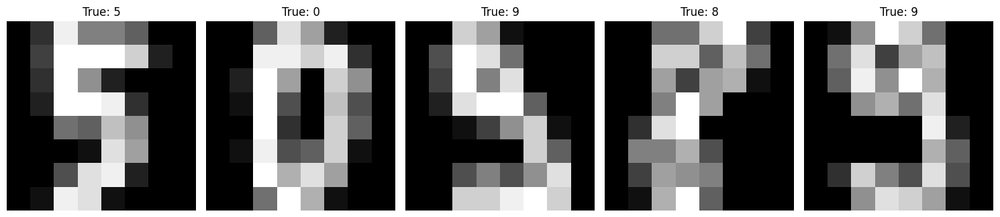
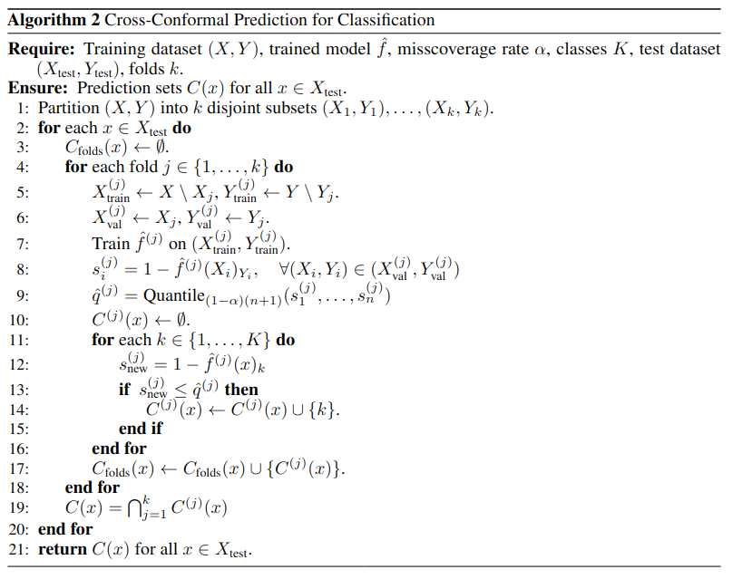
Alongside the maths and/or algorithms for each method, we will be exploring them through custom code implementations. In Full CP for classification, we will use a small version of the MNIST Digits dataset. You can see a few examples of handwritten digits below.
Really quickly before we explore the first method, see the performance of a standard neural network below. As you can see, the task/dataset is not a difficult one so the model excels.
Transductive CP#
Full Transductive Conformal Prediction (Full TCP) is the original and most rigorous variant of CP. Full TCP re-trains the model for each test instance and for each possible class, augmenting the training data with the new data point each time Yes! That means the neural network is reinitialized and trained \( |X_{test}| \cdot K \) times! As you can tell, this is incredibly computationally expensive.
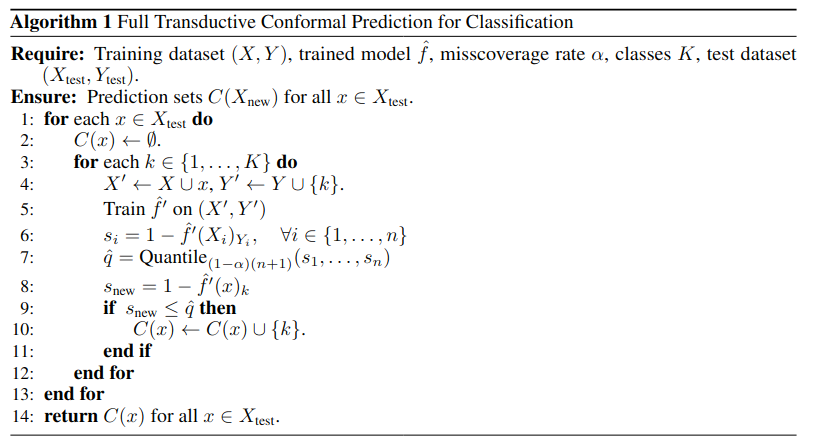
You can see the full Algorithm for Full TCP above, but it is simpler than it looks. It loops over each data point in the test dataset \( x \in X_{test} \) and then each class \( k \in K \), this is to systematically test if each class could be in the prediction set at the end. First, the test point \( x \) is added to the training data with the current class \( k \) that we are checking in this instance of the loop:
$$ X’ \leftarrow X \cup x:,: Y’ \leftarrow Y \cup {k} $$
Then a new model \( \hat{f}’ \) is trained using the new augmented training dataset \( (X’, Y’) \). This new model assumes \( x \) truly belongs to the class \( k \), it does this to check whether \( x \) belonging to \( k \) makes sense with past observations in the unaugmented training dataset next. It now computes the conformity scores for each data point in the unaugmented training dataset. Then as expected, the quantile \( \hat{q} \) is computed using these conformity scores. Finally, the conformity score for the test data point \( x \) is computed:
$$ s_{new} = 1 - \hat{f}’(x)_k $$
This tells us how typical it would be for the test point \( x \) to have the label \( k \). The label \( k \) is then added to the prediction set if \( s_{new} \leq \hat{q} \). Then after looping through the remaining class labels \( k \in K \), we are left with the prediction set \( C(x) \).
That’s it! It’s pretty simple really. Full TCP just trains a new model to see what it would be like if the test point belonged to a certain class. Then if this seemed pretty plausible, it can be added to the prediction set.
The code pretty much follows the Algorithm to a tee. Remember to check out my GitHub repo for the full implementation.
for test_idx in range(len(x_test_limited)):
prediction_set = []
for candidate_label in range(num_classes):
x_train_aug = np.vstack([x_train, x_test_point])
y_train_aug = np.vstack([y_train, tf.keras.utils.to_categorical([candidate_label], num_classes=num_classes)])
model_aug = get_model()
model_aug.compile(optimizer='adam', loss='categorical_crossentropy', metrics=['accuracy'])
model_aug.fit(x_train_aug, y_train_aug, epochs=epochs, batch_size=batch_size, verbose=0)
nonconformity_scores = compute_nonconformity_score(model_aug, x_train, y_train)
q_hat = np.quantile(nonconformity_scores, (1 - alpha))
test_point_nonconformity = compute_nonconformity_score(model_aug, x_test_point, tf.keras.utils.to_categorical([candidate_label], num_classes=num_classes))
if test_point_nonconformity <= q_hat:
prediction_set.append(candidate_label)
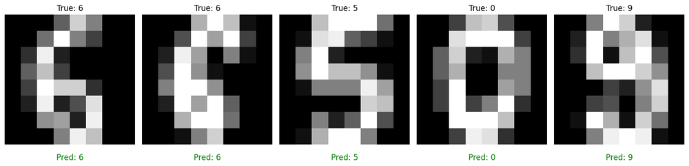
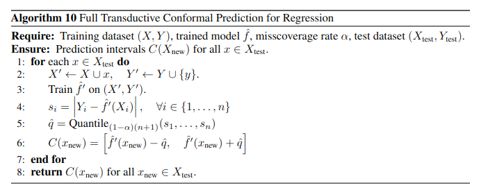
sorted_prediction_set = prediction_setIf we then test Full TCP on our MNIST dataset, we can actually see that some images come with some uncertainty, which was not visible with the base neural network. For example, for the second image, the model originally predicted “6” (which is correct). But using Full TCP, we find out that the model thinks “4” and “8” are also plausible, which looking at the image, seems to make sense as the image is a little deformed.
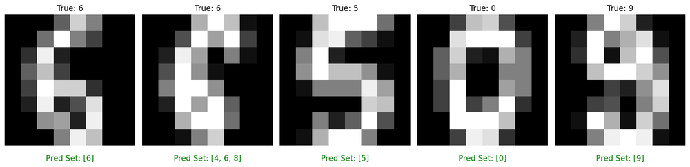
In fact, I printed out some other metrics so you could see how Full TCP changes predictions. Across the full test dataset, the average prediction set size was 1.14. This tells us that Full TCP returns singletons when the model is extremely confident, but there are a few edge cases where the model is a little less certain than we expect. We also achieved 100% accuracy, as the true label was within the prediction set in every test dataset point.
That is it, to recap Full TCP retrains the model for each class for each test dataset point. This is where the major drawback lies, I used a small neural network and a subsample of the actual test dataset (50 data points) and this code took \( \approx 40 \) minutes to run on a powerful machine! This method becomes pretty much infeasible if you have a larger neural network.
Cross CP#
Because Full TCP is computationally expensive, it needs to train a new model for every test point and every label, researchers developed Cross CP. Instead, Cross CP leverages k-fold cross-validation to reduce the number of times a new model needs to be trained. For every test point, a new model is trained \( k \) times (depending on how many k-folds a user specifies). For example, given a test dataset with 10 data points and 10 classes, Full TCP will train a new model \( 10 \cdot 10 = 100 \) times. In Cross CP, if we specify 5 k-folds, then it reduces the number of times we train a new model to \( 10 \cdot 5 = 50 \) times. Evidently, this allows Cross CP to be far more scalable to large-scale tasks than Full TCP.
You can see the full Algorithm for Cross CP above, it builds on Full TCP quite simply. It loops over each data point in the test dataset \( x \in X_{test} \) and then each fold in the specified k-folds. It then splits that fold’s data in train and validation split, then trains a new model \( \hat{f}^{(j)} \) on that train split. The conformity scores are then computed on the validation split of the k-fold, and the quantile \( \hat{q} \) is calculated straight after.
Next, it loops over each possible class \( K \) and computes the conformity score for the test point belonging to that class, it then adds it to the prediction set for that fold accordingly. This is where the folds get interesting, the final prediction set is then the intersection of all fold-wise prediction sets:
$$ C(x) = \cap^{k}_{j=1} C_{(j)}(x) $$
This is a little conservative in nature, to show why let’s run through a tiny example. If fold 1’s prediction set is {Cat} and fold 2’s prediction set is {Cat, Rabbit}, then the final prediction set using this intersection will be {Cat}. For a class to be in the final prediction set, the belief for the class must hold over all folds. As we will see in some mock experiments later, this conservative can be a small issue.
And that is it! Cross CP reduces the number of newly trained models by leveraging cross-validation. The code is actually simpler than the math makes it look.
for test_idx in range(len(x_test_limited)):
        prediction_sets_per_fold = []
        for train_index, val_index in kf.split(x_train):
            x_train_fold, x_val_fold = x_train[train_index], x_train[val_index]
            y_train_fold, y_val_fold = y_train[train_index], y_train[val_index]

            model = get_model()
            model.compile(optimizer='adam', loss='categorical_crossentropy', metrics=['accuracy'])
            model.fit(x_train_fold, y_train_fold, epochs=epochs, batch_size=batch_size, verbose=0)

            nonconformity_scores = compute_nonconformity_score(model, x_val_fold, y_val_fold)

            fold_prediction_set = []
            for candidate_label in range(num_classes):
                test_point_nonconformity = compute_nonconformity_score(model, x_test_point, tf.keras.utils.to_categorical([candidate_label], num_classes=num_classes))

                q_hat = np.quantile(nonconformity_scores, 1 - alpha)
                if test_point_nonconformity <= q_hat:
                    fold_prediction_set.append(candidate_label)

            prediction_sets_per_fold.append(set(fold_prediction_set))

        final_prediction_set = set.intersection(*prediction_sets_per_fold)
        sorted_prediction_set = sorted(final_prediction_set)
We can now test Cross CP on the MNIST dataset again, and compared to Full TCP, Cross CP is definitely more conservative. The second image in Full TCP we saw has a prediction set size of 3, but now this has been reduced to 1. This is still correct, and I guess more efficient, but since this is an approximation of Full TCP, then this is clearly conservativeness not confidence in the prediction.
Again, I printed out other metrics to see how well it performs. Across the full test dataset, the average prediction set size was 1.04 which is lower than Full TCP. However, the conservativeness is clearly harmful in some predictions as the method has an accuracy of 98%.
To recap, Cross CP reduces computation in comparison to Full TCP by retraining a model for each test point for each k-fold. This allows it to be more scalable as a user can effectively use a cost of the computation power needed, albeit at the cost of efficacy. With the same neural network as Full TCP, on a subsample of the actual test dataset (50 data points), this code took \( \approx 20 \) minutes to run using 5-folds on a powerful machine! So we cut the computation time in half! That is pretty impressive for the trade-off of one incorrect prediction.
Approximate CP#
Approximate CP is a very new paper/method that caught my eye in the list of accepted papers at ICLR ‘25, a conference I reviewed for. Approximate CP (ACP) tries to tackle the same issue as Cross CP, approximating Full TCP as accurately as possible whilst reducing the computation and improving scalability, but the solution it comes to is extremely unique and novel. Unlike Full TCP and Cross-CP, ACP trains the model a singular time and uses the Gauss-Newton influence to approximate the effect of retraining the model with the new test label.
You can see the full Algorithm for ACP above. Yes, it looks extremely daunting, but I will try to break it down as simply as possible. So, ACP first starts by training a model \( \hat{f} \) on the training dataset. Typically, in other Full CP methods, the model is retrained for every possible test example but this doesn’t happen here. Instead, ACP takes a shortcut by first computing an approximate inverse hessian on the train data:
$$ H^{-1}_{\text{GN}} = \frac{1}{n} \sum_{i=1}^{n} \left( \nabla_{\theta} \ell(Y_i, \hat{f}(X_i)) \right)^2 + \lambda I $$
I think the simplest way of explaining what this does is to compare it to a sensitivity map. It will allow us later to estimate how much the model parameters would change if we retrained it on a new test example without actually retraining it. Then, for each test point and each class label \( k \), it computes the gradient of the loss. Using the inverse hessian computed earlier, this then tells it how much the model’s parameters \( \theta \) would change if the test example was added to the dataset:
$$ \Delta \theta = H^{-1}_{\text{GN}} g_{\text{test}} $$
The conformity score is then defined as how much the model’s decision would change given the new test point possibly belonging to the class \( k \). This is a little different to how conformity scores have been computed in previous methods. The test points conformity score \( s_{new} \) is then compared to the scores from the train dataset to compute a p-value, this decides if the class \( k \) is added to the prediction set. If a high p-value is returned, it means the model is not surprised by this class label, so it is added to the prediction set. If a low p-value is returned, the model is surprised by this class label, so it is excluded.
Hopefully, this breaks it down a little easier so that it is understandable. ACP leverages influence functions to approximate conformity without retraining the model more than once. This allows ACP to scale a lot larger than previous methods discussed.
Since this paper was still under review at the time of writing this post, no official repository was given. So, I had to create the method myself with no guide except the paper, therefore it isn’t optimized very well. You can see it implemented below.
def compute_hessian_inverse_approx_diagonal(base_model, x_train, y_train):
    hessian_diag = None
    for i in range(len(x_train)):
        with tf.GradientTape() as tape:
            prediction = base_model(x_train[i:i+1], training=False)
            loss = tf.keras.losses.categorical_crossentropy(y_train[i:i+1], prediction)
        gradient = tape.gradient(loss, base_model.trainable_weights)
        flat_gradient = tf.concat([tf.reshape(g, [-1]) for g in gradient], axis=0)
        if hessian_diag is None:
            hessian_diag = tf.square(flat_gradient)
        else:
            hessian_diag += tf.square(flat_gradient)
    hessian_diag /= len(x_train)
    hessian_inv_diag = 1.0 / (hessian_diag + 1e-5)  # Add small epsilon for numerical stability
    return hessian_inv_diag

def compute_indirect_influence_score(test_point, candidate_label, base_model, hessian_inv_diag, num_classes=10):
    candidate_label_one_hot = tf.keras.utils.to_categorical([candidate_label], num_classes=num_classes)
    with tf.GradientTape() as tape:
        prediction = base_model(test_point, training=False)
        loss = tf.keras.losses.categorical_crossentropy(candidate_label_one_hot, prediction)
    test_gradient = tape.gradient(loss, base_model.trainable_weights)
    flat_test_gradient = tf.concat([tf.reshape(g, [-1]) for g in test_gradient], axis=0)
    hessian_inv_diag = tf.reshape(hessian_inv_diag, [-1])
    parameter_adjustment = hessian_inv_diag * flat_test_gradient
    adjusted_loss = tf.reduce_sum(parameter_adjustment * flat_test_gradient)
    return float(adjusted_loss)

base_model = get_model()
base_model.compile(optimizer='adam', loss='categorical_crossentropy', metrics=['accuracy'])
base_model.fit(x_train, y_train, epochs=epochs, batch_size=batch_size, verbose=0)
hessian_inv_approx = compute_hessian_inverse_approx_diagonal(base_model, x_train, y_train)

with tqdm(desc="Processing images", unit="image") as pbar:
    for test_idx in range(len(x_test_limited)):
        prediction_set = []
        for candidate_label in range(num_classes):
            test_nonconformity_score = compute_indirect_influence_score(x_test_point, candidate_label, base_model, hessian_inv_approx)
            num_greater_equal = 0
            for i in range(len(x_train)):
                train_nonconformity_score = compute_indirect_influence_score(x_train[i:i+1], np.argmax(y_train[i]), base_model, hessian_inv_approx)
                if train_nonconformity_score >= test_nonconformity_score:
                    num_greater_equal += 1
            p_value = num_greater_equal / (len(x_train) + 1)
            if p_value > alpha:
                prediction_set.append(candidate_label)
        sorted_prediction_set = prediction_set
Due to this, I was only able to run the predictions for the example images below and not the whole dataset. We can see that ACP prints the same predictions and set sizes as Cross CP. If you can manage to optimize my code above, I urge you to run it and get in touch with me!
To recap, ACP is a new method to approximate Full TCP with less computation than both Full TCP and ACP. It is the most scalable method we have spoken about so far, and uses the Gauss-Newton influence method to approximate model retraining.
Split CP#
As I said earlier, conformal prediction can be split into two categories: Full and Split CP. We have just covered Full CP and relevant algorithms, and now we will dive into Split CP. Unlike Full CP which uses a leave-one-out approach, Split CP uses a calibration dataset. The train dataset is then used to simply train the model, and then the calibration dataset is used to compute the conformity scores. This means we don’t have to have to retrain the model, making Split CP a computationally efficient variant of conformal prediction. This comes at a small cost of slightly looser coverage guarantees, however, it is the most deployable/usable variant of conformal prediction. In this section, we will explore Split CP in detail, along with key methods that attempt to improve upon each other.
Alongside the maths and/or algorithms for each method, we will be exploring them through custom code implementations just like in the Full CP section. In the Split CP for classification, we will use the ImageNet dataset as we can now scale the experiments we do to get a better view of each method’s performance. You can see a few examples of images in the dataset below.
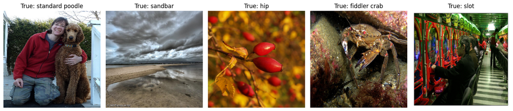
For these experiments, I used a pre-trained VGG19 model that was trained on the ImageNet dataset from the Keras developers. The model achieved a reasonable 66.12% accuracy on the test dataset and you can see a few examples below. In a way, this low accuracy is perfect as it will really show you the power of some of these methods!
Inductive CP#
Split Inductive Conformal Prediction (Split ICP) is the original lightweight conformal prediction variant that utilizes a holdout set. Instead of retraining the model for each test instance, and each class to compute conformity scores, Split ICP uses a holdout/calibration dataset to compute conformity scores instead. Whilst doing this alleviates a lot of computational power, it also requires removing some data from the training dataset or acquiring a new amount of data points from somewhere. The more data in the calibration dataset, the better calibrated the conformal prediction process is, the less data, the easier it is to acquire the data but the less calibrated the process will be.
See the Split ICP Algorithm above. As you can see, Split CP methods are separated into three steps. The first step is to train the base model \( \hat{f} \) on the training dataset. The second step is to compute the conformity scores. To do this, it iterates over the calibration dataset and computes the desired conformity scores \( s_i \) that the user specifies. In the algorithm and code, we use one minus the softmax score of the true label. Once it has iterated over the whole dataset, the threshold \( \hat{q} \) can be calculated. The final step is to construct the prediction sets for the test points by iterating over the test dataset and including all classes \( k \) whose softmax score is above \( 1 - \hat{q} \).
That is the entirety of Split ICP. As you can see, it is much lighter but it is very dependent on the quality and/or quantity of the calibration data. The code is also split up into three steps. Remember to check out my GitHub repo for the full implementation.
for batch_images, batch_labels in calibration_dataset:
    preds = model.predict_on_batch(batch_images)
    true_label_probs = preds[np.arange(len(batch_labels)), batch_labels.numpy().astype(int)]

    nonconformity_scores = 1 - true_label_probs
    calibration_scores.append(nonconformity_scores)

calibration_scores = np.concatenate(calibration_scores)

alpha = 0.05
n = len(calibration_scores)
q_level = np.ceil((n + 1) * (1 - alpha)) / n
q_hat = np.quantile(calibration_scores, q_level, interpolation="higher")
The second step (above), iterates over the calibration dataset and computes the desired conformity scores. It then computes the threshold \( \hat{q} \) afterwards. The final step (below), adds each class to the prediction set if the softmax score is higher than \( 1 - \hat{q} \).
for batch_images, batch_labels in test_dataset:
train_pred = model.predict_on_batch(batch_images)
for i in range(len(batch_images)):
true_label = batch_labels[i]
preds = train_pred[i]
prediction_set = np.where(preds >= 1 - q_hat)[0]
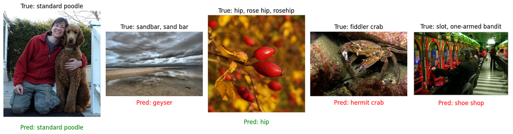
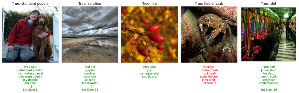
sorted_prediction_set = prediction_set[np.argsort(-preds[prediction_set])]We can then test Split ICP on the ImageNet test dataset to test its full potential. For all the example images below, Split ICP predicts multiple classes in the set. For some images (e.g., fifth image), the prediction set is large yet the actual class is still not contained within it.

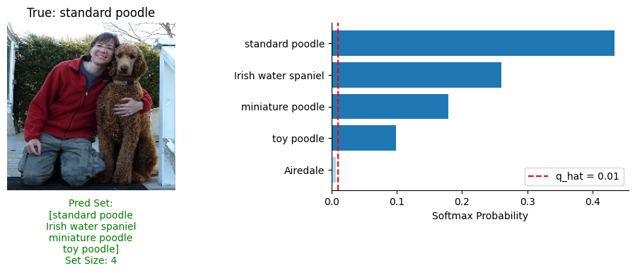
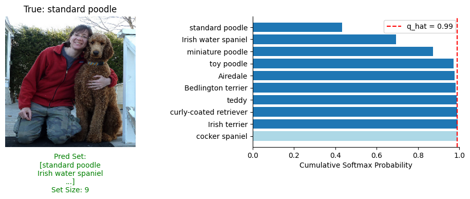
An example of how the prediction sets were created is displayed below. As you can see on the right of the image, the threshold \( \hat{q} \) is at 0.01, so the four most probable classes that sit above the threshold are included within the set.
For further metrics, Split ICP outputs an average prediction set size of 5.74 which proves it does actually adapt to some uncertainty- though clearly not enough. It has a top-5 accuracy of 86.11%, a top-10 accuracy of 89.71% and a coverage of 91.05%. Given that the base model had an accuracy of 66.12%, it shows that Split ICP does actually help which is fantastic! Where Full TCP took 40 minutes to output prediction sets for 50 MNIST images, Split ICP only takes 23 minutes to output prediction sets for 40,000 ImageNet images! This is the best empirical analysis of how lightweight Split CP methods are! Another flaw of the Split CP method is highlighted in this experiment. We specify a 95% coverage (\( \alpha=0.05 \)) rate, however, Split ICP only achieves a coverage of 91.05%. This is an \( \approx 4% \) extra misscoverage rate. Split CP methods have much looser coverage guarantees as they rely heavily on the calibration dataset quantity/quality and the model itself.
If we specify a 90% coverage (\( \alpha=0.1 \)) rate, Split ICP has an average prediction set size of 2.60 and a coverage of 84.25%. This is again, way lower than the specified misscoverage rate.
To recap, Split ICP computes conformity scores on a calibration dataset. This allows it to be a computationally efficient variant of conformal prediction, at the cost of some coverage guarantees. The scalability of this method is only proven in the large-scale experiments we performed above.
Adaptive Prediction Sets#
As efficient as Split ICP is, it can be conservative and not flexible as it applies a single threshold \( \hat{q} \) to all test points. Adaptive Prediction Sets (APS) aims to improve upon these points and provide more accurate coverage guarantees by computing…well…adaptive prediction sets for each test point by progressively accumulating class probabilities in descending order until the total probability mass surpasses the required threshold \( \hat{q} \).
As seen in the APS Algorithm above, the first two steps are the same as in Split ICP. Where it improves upon Split ICP is within the third step. Instead naively of including all classes about the threshold \( \hat{q} \), APS first sorts the softmax probabilities from largest to smallest for all classes \( k \) to calculate the cumulative probabilities. Each class is then included within the prediction set until the cumulative probability of the included classes exceeds the threshold \( \hat{q} \) (note: the class that exceeds the threshold is included).
It’s quite a simple change to the Split CP approach, but as you will see with the empirical tests, it has quite a large effect. Remember to check out my GitHub repo for the full implementation.
for batch_images, batch_labels in test_dataset:
    train_pred = model.predict_on_batch(batch_images)

    for i in range(len(batch_images)):
        true_label = batch_labels[i]
        preds = train_pred[i]

        sorted_indices = np.argsort(-preds)
        sorted_preds = preds[sorted_indices]
        cumulative_probs = np.cumsum(sorted_preds)

        prediction_set_size = np.searchsorted(cumulative_probs, q_hat) + 1
        sorted_prediction_set = sorted_indices[:prediction_set_size]
Again, the code doesn’t change much. The predicted softmax scores get sorted in descending order and get cumulative summed. Then the classes can be added into the prediction set until the cumulative probability is above the threshold.
When we test APS on the ImageNet dataset, we can see it produces a lot larger prediction sets than Split ICP. For example, the fifth image in Split ICP struggled to include the true label in the prediction set due to it applying a single threshold to all test points. APS adapts its behaviour dynamically to each image and increases the prediction set size due to large amounts of uncertainty. This creates a very large prediction set (284 classes included) but it means the true label is within the set and it indicates how uncertain it is.

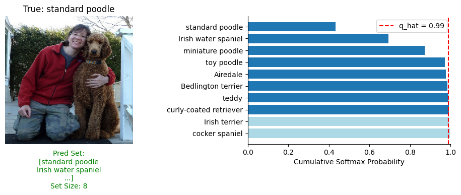
We can see how the prediction sets get created differently to Split ICP. On the right of the image below, each class is included in the prediction set until “Irish terrier” exceeds the threshold.
In terms of performance, APS predicts an average set size of 75.11. This is a massive increase compared to Split ICP’s 5.74! But with this, it achieves a final coverage of 98.11% compared to 91.05% when using \( \alpha=0.05 \). One of Split ICP’s flaws was a struggle to achieve the specified coverage rate, APS can achieve it using the adaptive technique.
To recap, APS builds upon Split ICP by including classes in the prediction set based upon a cumulative probability instead of the naive thresholding technique for each individual class. This means APS can achieve a better coverage guarantee with little extra computation.
Regularized Adaptive Prediction Sets#
Regularized Adaptive Prediction Sets (RAPS) acknowledges that APS can achieve better coverage but at the cost of larger than necessary prediction set sizes. The aim of this method was to achieve the same great coverage but reduce the size of the prediction sets. To do this, RAPS regularizes the prediction probability distribution to encourage the exclusion of unreliable probabilities at the tail. During the empirical tests, we will see how this works in action compared to APS.
The RAPS Algorithm can be seen above. RAPS requires two new parameters, a regularization parameter \( \lambda \) and a regularization amount \( k_{reg} \). Just like Split ICP and APS, training the model and computing the calibration conformity scores remains the same. After the threshold \( \hat{q} \) is calculated, RAPS calculates the regularization \( r \) that determines how the regularization affects probabilities. The top labels, determined by the regularization amount \( k_{reg} \), are assigned 0 which means they will not be affected by the RAPS process. The next \( K - k_{reg} \) labels are assigned a tuneable regularization parameter \( \lambda \), this is used to manually inflate the associated label probabilities. This will allow RAPS to hopefully reduce prediction set sizes by excluding low probability classes by inflating their probabilities so they sit over the threshold \( \hat{q} \) sooner.
During step 3, where the prediction sets are calculated for each test data point, the model predicts upon the test point and the probabilities are sorted in descending order- as seen in APS. The regularization \( r \) is then added to the sorted probabilities \( \hat{p}_{sorted} \) to forcibly inflate the probabilities at the tail of the prediction set. Then the regular process occurs as we saw in RAPS. The probabilities are cumulatively summed, and then the classes \( k \) are added to the prediction set until the cumulative probability exceeds the threshold \( \hat{q} \).
As you will see, this small change greatly affects the results. Remember to check out my GitHub repo for the full implementation.
lambda_reg = 0.001
k_reg = 5
num_classes = 1000
reg_vec = np.array(k_reg * [0,] + (num_classes - k_reg) * [lambda_reg,])[None,:]

for batch_images, batch_labels in test_dataset:
    train_pred = model.predict_on_batch(batch_images)

    for i in range(len(batch_images)):
        true_label = batch_labels[i]
        preds = train_pred[i]

        sorted_indices = np.argsort(-preds)
        sorted_preds = preds[sorted_indices]

        sorted_preds_reg = sorted_preds + reg_vec.squeeze()
        sorted_preds_reg_cumsum = sorted_preds_reg.cumsum()

        _ind = (sorted_preds_reg_cumsum - sorted_preds_reg) <= q_hat
        sorted_prediction_set = sorted_indices[_ind]
In the code, we first calculate the regularization vector \( r \) using \( \lambda, \medspace k_{reg}, \text{and} \medspace K \). The only addition after that is adding this vector onto the sorted predictions to artificially inflate the probabilities.
When tested on the ImageNet dataset, RAPS effectively manages to reduce the size of the prediction sets considerably whilst still including the true label within the prediction set in comparison to APS. For example, the fifth image had a prediction set size of 284 in APS, but RAPS reduced this to 69 whilst still including the true label!
If we see how the prediction sets get created on an example image, we can visually see the effect of the regularization process. Where APS included “Irish Terrier”, RAPS excluded this as it has a very low probability and was increased to above the threshold.
When we look at the overall performance of RAPS, it achieves an average set size of 21.09. This is a massive drop compared to APS which had an average size of 75.11. It also achieves a coverage of 96.27% when using \( \alpha=0.05 \) and \( \lambda=0.001 \), whilst APS achieved 98.11%. What we can take away from this is using a regularized approach to crafting prediction sets achieves the same correct coverage rate but with a massive drop in prediction set size.
We can also test out \( \lambda \) effects performance. If we use \( \lambda=0.01 \), we get a coverage of 93.18% with an average set size of 8.79. While if we switch to \( \lambda=0.0001 \), we get a coverage of 97.65% and an average set size of 45.35. Based on this, it is clear that over-regularization can be a problem. When \( \lambda \) is set too high, RAPS does not achieve the specified coverage. When we under-regularize, RAPS hits coverage and still produces considerably lower set sizes than APS. Evidently, I think it is safe to say under-regularization is not an issue as it will achieve APS-level results or better!
To recap, RAPS builds upon APS by artificially boosting the probabilities of the tail of the prediction set. This allows RAPS to achieve coverage whilst significantly reducing prediction set size.
Monte-Carlo Conformal Prediction#
Monte-Carlo Conformal Prediction’s (MC-CP) problem statement is that even RAPS can produce larger than necessary set sizes, therefore, it attempts to build upon this and reduce them further. MC-CP combines RAPS and a proposed approximate Bayesian inference (Adaptive MC Dropout) to reduce the tail probabilities that are less likely and boost the head probabilities that are more likely.
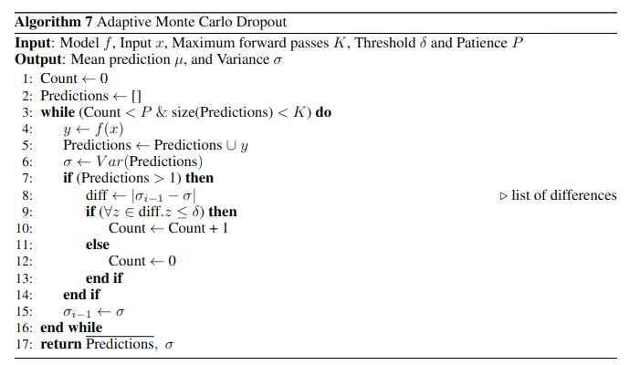
If the conformal prediction procedure is combined with approximate Bayesian inference like Monte-Carlo Dropout, it would be computationally expensive as MC-Dropout performs \( K \) forward passes with dropout layers in the network switched on. This allows the mean of the predictions to accurately reflect the uncertainty estimation by capturing the variability in predictions, leading to more reliable conformal prediction sets that reflect model confidence. In a somewhat well-calibrated model, this mean of the predictions would have boosted/stable probabilities at the head of sorted probabilities and reduced probabilities at the tail. But since this is computationally expensive, the authors of the paper created Adaptive Monte-Carlo Dropout, seen in the Algorithm above. Adaptive MC Dropout tracks the variance of the predictions at each forward pass. Once the variance stabilizes across all classes below a chosen threshold \( \delta \) for \( P \) consecutive forward passes, then the remaining \( k \) forward passes will provide little to no extra information than we already have. Therefore, the MC Dropout process is stopped early to save computation.
The full MC-CP Algorithm can be seen above. It is exactly the same as RAPS except the calibration and inference steps extract the mean probabilities from the Adaptive MC Dropout process seen earlier. Since there is not much else to detail from the method, we can skip straight to the code and results!
mc_preds = []
prev_variance = None
current_patience_count = 0
for j in range(num_mc_samples):
    preds = model(batch_image, training=True)
    mc_preds.append(preds)
    if len(mc_preds) > 1:
        current_variance = np.std(mc_preds, axis=0)
            if prev_variance is not None:
               var_diff = np.abs(current_variance - prev_variance)
               if np.all(var_diff <= delta):
                    current_patience_count += 1
               else:
                    current_patience_count = 0
               if current_patience_count >= patience:
                    break

        prev_variance = current_variance

mc_preds = np.array(mc_preds)
mean_preds = np.mean(mc_preds, axis=0)[0]
The code for the Adaptive MC Dropout process can be seen above. It iterates over the MC Dropout process until the variance stabilizes across all classes below a chosen threshold \( \delta \) for \( P \) consecutive forward passes or until the maximum forward passes \( K \) is reached.
Since I have made all of these tutorials on my home computer, and seen MC-CP can be computationally heavier than most other methods, I switched back to the MNIST dataset for this experiment. But for clarity’s sake, I re-ran RAPS on MNIST also for comparison.
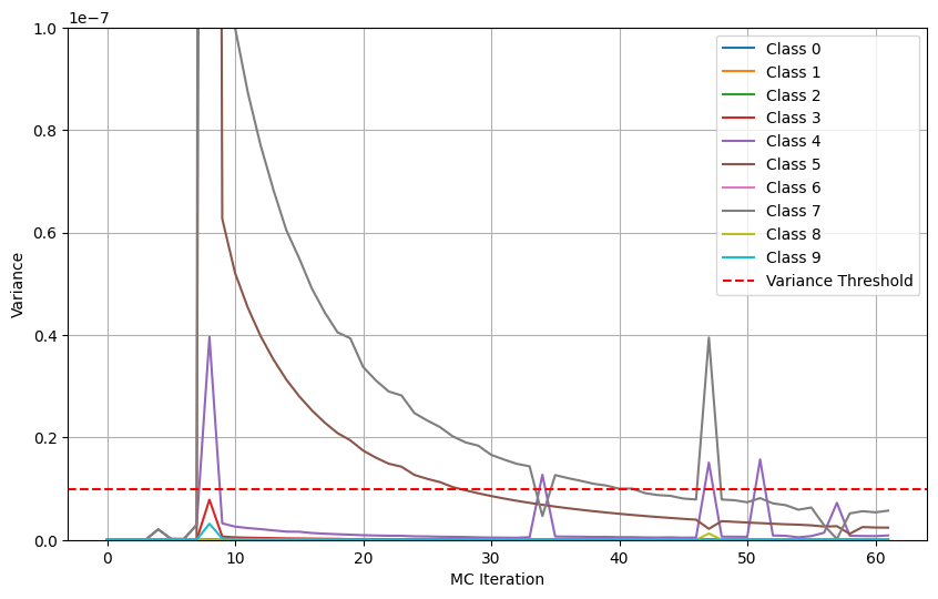
Above is an example visualization of the Adaptive MC Dropout process on an input of the digit ‘7’. As you can see variance of the predictions for possible classes (e.g., 5 and 7) are high for the first few dozen forward passes, meaning the model is fluctuating with how high the probability should be for these classes. We can also see that variance peaks at the eighth forward pass for low probability classes (e.g., 4, 3, and 9) and is then near zero for the rest, meaning for one forward pass the model thought the input could possibly be these classes. With a regular model, there is a chance with the RAPS method for the prediction set to include {7, 5, 4, 3, and 9} as they all have some probability. With MC-CP, since it takes the mean of the forward passes, these tail probabilities will be all but removed from the prediction set leaving only the most probable classes. (e.g., 5 and 7). Finally, once all the class variances stabilize around forward pass 52, they do not exceed the threshold again so the Adaptive MC Dropout process finishes early at forward pass 61.
When tested on the MNIST dataset, RAPS achieves a top-1 accuracy of 94%, a final coverage of 100%, and an average set size of 1.58. MC-CP achieves an average set size of 1.50. Even though this is a small experiment, MC-CP manages to remove tail probabilities in the prediction set!
To recap, MC-CP aims to remove tail probabilities from the prediction set by performing a computationally efficient variant of approximate Bayesian inference during the calibration and inference phases of conformal prediction.
Mondrian CP#
The final Split CP for classification method we will cover is Mondrian CP. Mondrian CP is an extension of Split ICP that aims to ensure valid coverage guarantees per class, this is most useful for datasets with large class imbalances, as it generates a threshold \( \hat{q}_k \) per class \( k \in K \) instead of one threshold \( \hat{q} \) for all classes.
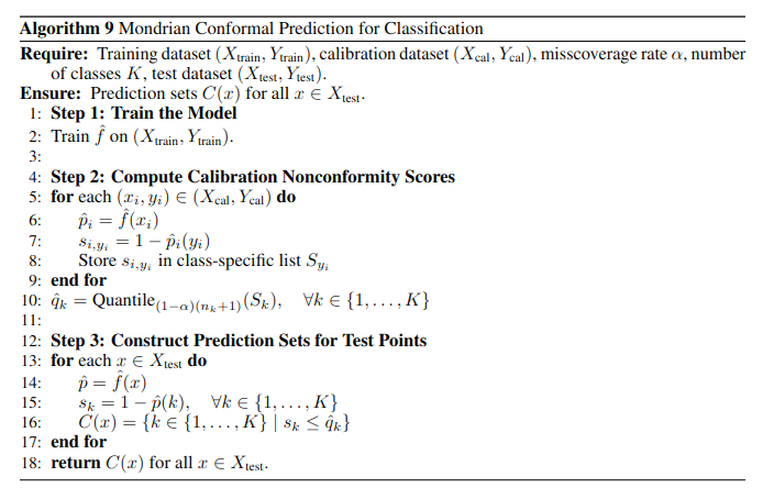
The Algorithm for Mondrian CP is not much different to Split ICP. When computing the calibration conformity scores, Mondrian CP stores \( s_i \) in a class-specific list according to the true label \( y_i \). Then, a quantile for each class \( \hat{q}_k \) can be computed for each class-specific list \( S_k \). This allows the methods to have better coverage control per class, potentially reducing under-coverage for rarer classes. During the inference step, the prediction sets are created by first computing a conformity score \( s_k \) for each class \( k \in K \). Then for each possible class label, the label is added to the prediction set if the conformity score sits below the respective class threshold \( \hat{q}_k \).
The code has a few tweaks from the Split ICP code. The calibration scores are added to class-specific lists.
for i, label in enumerate(batch_labels.numpy()):
    calibration_scores_per_class[int(label)].append(nonconformity_scores[i])
This then allows Mondrian CP to compute a class-specific threshold.
q_hat_per_class = {
    label: np.quantile(scores, 1 - alpha, method="higher")
    for label, scores in calibration_scores_per_class.items()
}
During the inference step, the class-specific conformity score is compared to the class-specific threshold. If the score is less than the threshold, then the label is added to the prediction set.
nonconformity_scores = 1 - preds

prediction_set_indices = []
for c in range(len(preds)):
    class_q_hat = q_hat_per_class.get(c, 1 - alpha)  # Get class-specific q_hat
    if nonconformity_scores[c] <= class_q_hat:
        prediction_set_indices.append(c)

sorted_prediction_indices = np.argsort(-preds[prediction_set_indices])
sorted_prediction_set = [prediction_set_indices[idx] for idx in sorted_prediction_indices]
When tested on the ImageNet dataset, Mondrian CP exhibits conservative behaviour. Due to each class-specific threshold, technically, having less data to use for calibration. As a result, Mondrian CP can sometimes fail to include the true label in the prediction set.

Visualizing how the prediction sets get created, we can see how confident Mondrian CP is for each class. Typically, a lower \( \hat{q} \) means the CP method is more confident in the predictions, whilst a higher \( \hat{q} \) means it struggles with classification. This extends to Mondrian CP and can now give us some interpretability about the underlying model’s prediction per class. In the example below, we can interpret that the CP process has found the model is more confident about the “Irish Water Spaniel” class than it is the “Miniature Poodle” class.
Since the model is so confident about the “Irish Water Spaniel” class, it takes a smaller conformity score for it to be excluded from the prediction set compared to the “Miniature Poodle” class.
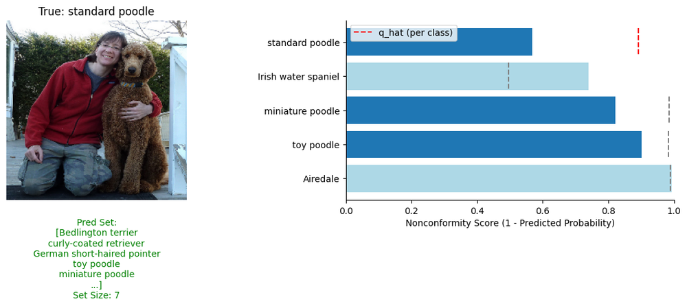
The overall performance of Mondrian CP reflects this same conservative behaviour. Mondrian CP has an average set size of 12.18 when using \( \alpha=0.05 \) and a final coverage of 85.93%. This is a large difference in misscoverage rate, especially when compared to the powerful performance of APS, RAPS, and MC-CP!
To recap, Mondrian CP extends upon Split ICP by attempting to guarantee class-specific coverage. Whilst this may work at times, it can also display conservative behaviour when crafting prediction sets.
Conformal Prediction For Regression#
Now we will do a deep dive into conformal prediction for regression tasks. Just like the classification method, we will cover state-of-the-art algorithms, the maths, and the code behind each one.
Full CR#
Full conformal regression is again, the rigorous variant of conformal prediction but applied to regression tasks. It again utilizes the leave-one-out approach to construct prediction sets, but there are quite a few unique nuances compared to what we saw in the previous classification modality. In this section, we will explore the classical Full CR method, the interesting tweaks we can make to improve Full CR, and alternative approaches designed to improve coverage and reduce prediction interval width.
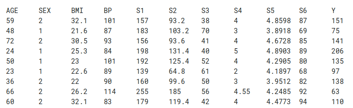
Alongside the maths and/or algorithms for each method, we will explore them through custom code implementations. In Full CR, we will use the small Diabetes dataset to compare and empirically run the implementations. You can see a print of some entries of the dataset below.
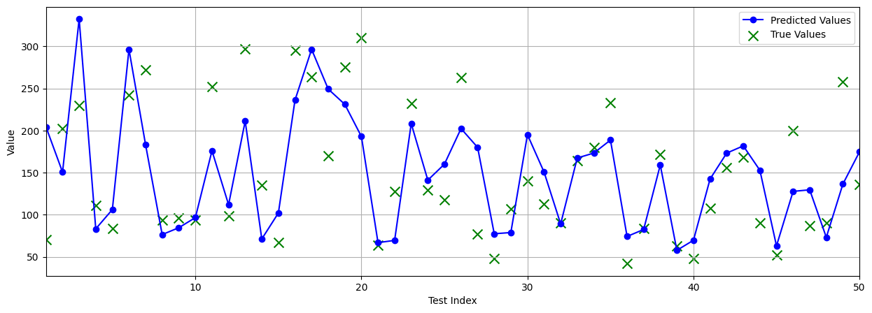
The performance of the standard neural network can be visualized below. It achieves a final mean absolute error (MAE) of 43.36 on the test dataset. While not a difficult dataset, and this performance can definitely be improved, I chose not to better showcase the CR methods that we will look at throughout.
Before we move on to the first method, we should talk about deep quantile regression (DQR) models, a popular type of neural network to combine with conformal regression. Instead of predicting a single point estimate (like in standard regression), the DQR model estimates different quantiles of the target distribution (e.g., 10th, 50th, and 90th percentiles ). This helps model uncertainty by capturing the full conditional distribution of the ground truth value.
This is typically the network of choice with conformal regression, though a standard regression model is perfectly viable, as conformal regression can refine the predicted quantile intervals by adding a statistical correction to ensure the desired coverage probability. This combination allows for robust uncertainty quantification alongside the flexibility of learning the quantiles.
output_layer = Dense(len(quantiles), activation='linear')(hidden)As seen above, the network outputs a node for each desired quantile. For example, if we want to estimate the 10th, 50th, and 90th quantiles, there will be three output nodes.
The network also requires a custom loss function to refine the outputs, as a simple mean squared error (MSE) term will not suffice. Below is an example of the asymmetric quantile-loss or pinball-loss that is used to train DQR models. This function applies different penalties for underestimation vs overestimation and then penalizes error asymmetrically based on the quantile level. This ensures the model learns to approximate the target quantiles rather than just the mean.
def quantile_loss(quantiles):
def loss(y_true, y_pred):
y_true_expanded = tf.expand_dims(y_true, axis=-1)
errors = y_true_expanded - y_pred
losses = []
for i, q in enumerate(quantiles):
error = errors[:, i]
loss_q = tf.maximum(q * error, (q - 1) * error) # Asymmetric quantile loss
losses.append(tf.reduce_mean(loss_q)) # Mean loss for each quantile
return tf.reduce_sum(losses) # Sum losses across quantiles
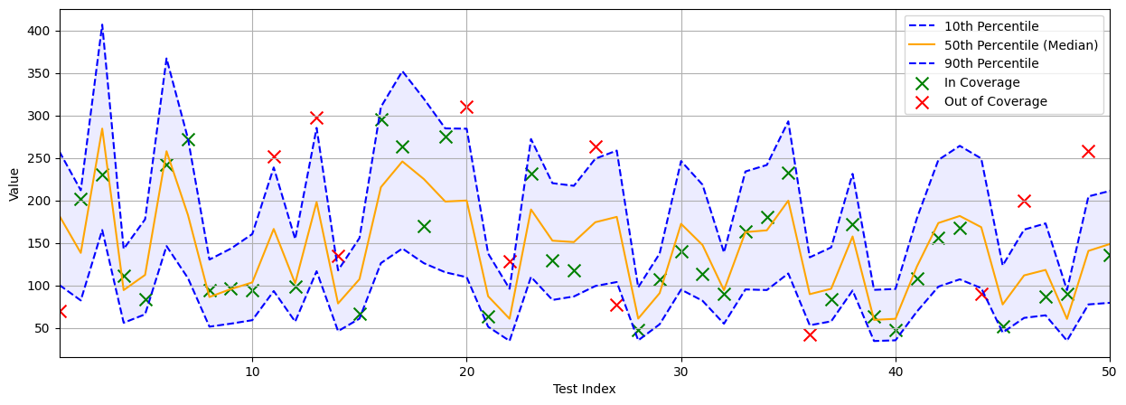
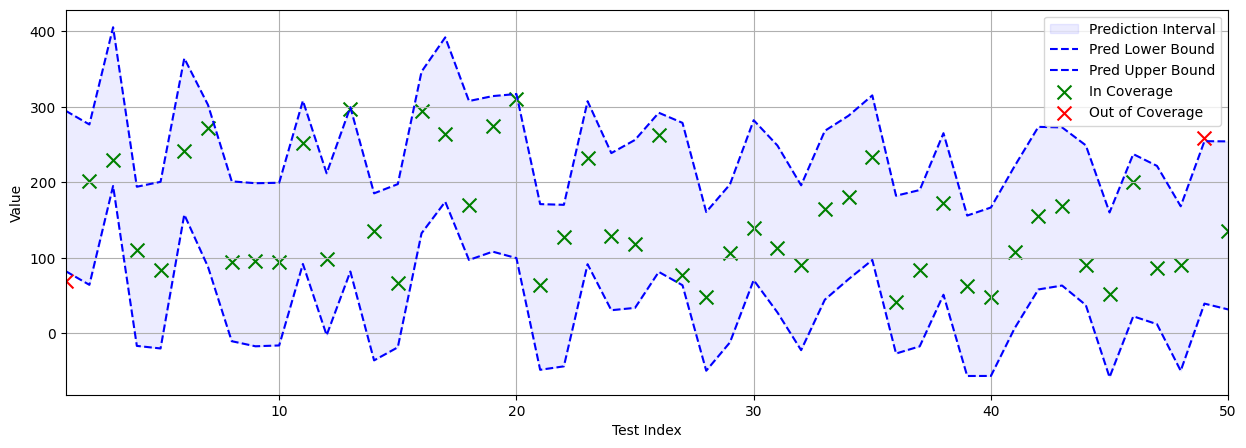
return lossThe performance of the deep quantile regression network can be visualized below. Instead of point estimates, the network predicts an interval between the top and bottom quantiles (in this case, 10th and 90th). With this type of network, the interval width at each test data point represents the uncertainty of the model- a smaller width represents greater certainty, and a larger width represents greater uncertainty. On the Diabetes test dataset, the model achieves a coverage of 74.16% with an average interval width of 126.35.
Transductive CR#
Full Transductive Conformal Prediction (Full TCP) for regression is, in essence, very similar to Full TCP for classification. For classification, the model is retrained for each test instance and for each possible class label \( k \). For regression, the model is only retrained for each test instance and we only have point estimates in regression. While this is, in a way, computationally slightly lighter, the burden of heavy computation still remains, unfortunately- albeit, not as exacerbated.
The Algorithm for Full TCP for regression can be seen above and shares parallels to classification but brings unique nuances which will act as the foundation for conformal regression. First, it loops over each data point in the test dataset \( x \in X_{test} \). The model is then trained using a leave-one-out approach on the training dataset combined with the current test point.
$$ X’ \leftarrow X \cup x, \medspace Y’ \leftarrow Y \cup {y} $$
The conformity scores can then be calculated for each data point in the unaugmented training dataset. In regression, the common conformity score is the absolute difference between the ground truth value and the model’s prediction. Then, the threshold \( \hat{q} \) can be computed using these conformity scores. Differently to classification, to craft a prediction interval in regression, the threshold is then minus-ed from the prediction of the test point \( \hat{f}’(x_{new}) - \hat{q} \) to craft the lower bound and plus-ed to the prediction of the test point \( \hat{f}’(x_{new}) + \hat{q} \) to craft the upper bound. Full TCP does this for each test point in the test dataset.
That is all there is to it. Full TCP for regression trains a new model for each test point, computes the conformity scores and threshold, and then uses this to craft the upper and lower bounds of the prediction interval.
The code for this method is also very simple to create. Remember to check out my GitHub repo for the full implementation.
for test_idx in range(len(x_test)):
    x_test_point = x_test[test_idx].reshape(1, -1)
    true_value = y_test[test_idx]

    x_train_aug = np.vstack([x_train, x_test_point])
    y_train_aug = np.hstack([y_train, [true_value]])

    model_aug = get_model(input_shape=x_train.shape[1])
    model_aug.compile(optimizer='adam', loss='mae')
    model_aug.fit(x_train_aug, y_train_aug, epochs=epochs, batch_size=batch_size, verbose=0)

    nonconformity_scores = compute_nonconformity_score(model_aug, x_train, y_train)
    q_hat = np.quantile(nonconformity_scores, 1 - alpha)

    prediction_lower = model_aug.predict(x_test_point, verbose=0)[0] - q_hat
    prediction_upper = model_aug.predict(x_test_point, verbose=0)[0] + q_hat
If we test Full TCP on the Diabetes dataset using a regular regression model, we can observe that it correctly crafts prediction intervals to measure uncertainty within the model and maintain desired coverage. Bar two points (visualized by red crosses), the majority of data points are included within coverage.
If we look at performance metrics when using \( \alpha=0.05 \), Full TCP achieves a final coverage of 96.63% which is above the desired coverage rate. It also achieves an average interval width of 213.38. So whilst it guarantees coverage, the width is quite large.
This is where we can utilize the deep quantile regression model mentioned earlier to calculate better-calibrated intervals. This requires two slight changes to the algorithm, the first being the conformity score. Instead of the conformity scores being the absolute difference between the ground truth value and the prediction, it is calculated as so:
$$ s_i = \max \left( 0, \max \left( \hat{y}_{i, \text{lower}} - Y_i, Y_i - \hat{y}_{i, \text{upper}} \right) \right), \quad \forall i \in {1, \dots, n} $$
This means if the ground truth value lies within the predicted interval, the score is 0 as it is considered conforming. Otherwise, the score is how far it sits outside the interval. The second change is how the prediction intervals are calculated:
$$ C(x_{\text{new}}) = \left[ \hat{y}_{\text{lower}}(x_{\text{new}}) - \hat{q}, \quad \hat{y}_{\text{upper}}(x_{\text{new}}) + \hat{q} \right] $$
Instead of adding and subtracting the threshold \( \hat{q} \) to the predicted point estimate, it is subtracted from the lower quantile \( \hat{y}_{lower} \) and added to the upper quantile \( \hat{y}_{upper} \).
When using a DQR model, Full TCP is better calibrated as the underlying model learns its own upper and lower quantiles and then Full TCP can add buffer to these quantiles to guarantee coverage, as you can see below!
Using a DQR model, Full TCP achieves a final coverage of 97.75% and an average interval width of 196.22. This is greater coverage and reduced than when using a base model, empirically backing up claims of better calibration. Computing prediction intervals of the Diabetes test dataset takes around \( \approx 11 \) minutes, showcasing how Full CP methods, once again, are computationally expensive.
To recap, Full TCP for regression retrains a model for each test data point. After computing the conformity scores and threshold, it removes and adds it to craft the upper and lower prediction interval bounds.
Split CR#
Split CR utilizes a calibration dataset instead of a leave-one-out approach. This makes it computationally faster, as we saw in the classification methods. This means that coverage is dependent on the size, balance, and quality of the calibration set.
We will be using the Diabetes dataset again, so no need to go over visualization and how the base model performs as it is all the same! From this point out, we will only use the quantile model for all experiments as it is considered the gold standard.
Conformalized Quantile Regression#
The first method we will look at in split conformal regression methods is Conformalized Quantile Regression (CQR). Just like all Split CR and CP methods, CQR is a three-step approach that utilizes a calibration dataset to compute conformity scores instead of retraining the model for every test point.
The Algorithm for CQR can be seen above. The first step is to train the deep quantile regression model on the train dataset based on the user’s specified quantiles \( \tau \). This will be the only time the model is training as this is a Split CR method. The second step is to compute the conformity scores on the calibration dataset. CQR loops over the calibration dataset \( (x_i, y_i) \in (X_{cal}, Y_{cal}) \), and retrieves the models predicted quantiles for the \( i- \)th data point. The conformity score \( s_i \) is computed based on whether the ground truth value sits within the predicted interval. The final part of the calibration step is to compute the threshold \( \hat{q} \). The final step is to construct the prediction intervals for each test point. The predicted quantiles are retrieved from the model, specifically the lowest and highest quantiles are needed. The prediction interval is then calculated as the lowest quantile minus the threshold \( \hat{y}_{lower} - \hat{q} \) and the upper quantile plus the threshold \( \hat{y}_{upper} + \hat{q} \).
So, CQR is quite simple. It is basically a Split CP variant of transductive CP with a deep quantile network. The code is also split up into three steps. Remember to check out my GitHub repo for the full implementation.
for i in range(len(x_cal)):
    x_cal_point = x_cal[i].reshape(1, -1)
    true_value = y_cal[i]

    y_pred_quantiles = model.predict(x_cal_point, verbose=0)
    y_pred_lower = y_pred_quantiles[0, 0]  # 10th percentile
    y_pred_upper = y_pred_quantiles[0, 2]  # 90th percentile

    nonconformity_score = max(0, max(y_pred_lower - true_value, true_value - y_pred_upper))
    calibration_scores.append(nonconformity_score)

calibration_scores = np.array(calibration_scores)

alpha = 0.05
q_hat = np.quantile(calibration_scores, 1 - alpha)
The second step (above), iterates over the calibration dataset and computes the desired conformity scores. It then computes the threshold \( \hat{q} \) afterwards. The final step (below), crafts the calibrated/conformalized quantiles as stated in the algorithm.
for test_idx in range(len(x_test)):
    x_test_point = x_test[test_idx].reshape(1, -1)
    true_value = y_test[test_idx]

    y_pred_quantiles = model.predict(x_test_point, verbose=0)
    y_pred_lower = y_pred_quantiles[0, 0] - q_hat  # Adjusted 10th percentile
    y_pred_median = y_pred_quantiles[0, 1]         # 50th percentile (median)
    y_pred_upper = y_pred_quantiles[0, 2] + q_hat  # Adjusted 90th percentile
If we then test CQR on the Diabetes test dataset, we can see how it performs. Based of the visualization of the predicted quantiles below, it can be seen that CQR correctly adapts the quantiles to attempt to include as many data points in coverage as possible whilst attempting to keep interval widths as low as possible.

For full performance metrics, CQR achieves a final coverage of 94.38% when using \( \alpha=0.05 \). This is slightly under coverage to what we specified, but only a marginal amount. Really, this showcases how Split CP methods have looser coverage guarantees than Full CP methods. Since the Diabetes dataset is quite small, the likelihood is that there were not enough diverse data points to ensure coverage. CQR also achieves a final average interval width of 203.77.
Remember, Split CP methods are computationally lighter than Full CP methods. Where Full TCP took \( \approx 11 \) minutes to run, CQR took \( \approx 15 \) seconds to train, calibrate, and infer upon (the full CQR process)! This is a ridiculous amount of savings in terms of computation and time!
To recap, CQR is the base Split CR method that utilizes deep quantile networks and the Split CP methodology to reduce computation and time to perform conformalised regression.
Locally Adaptive CQR#
A similar issue that we saw in Split CP was that each test point was given the same threshold \( \hat{q} \). This issue remains in CQR. Locally Adaptive CQR (originally coined SLCR) attempts a similar approach to APS (in Split CP for classification) which is to build a method that creates a \( \hat{q} \) for each test point, evidently, dynamically adapting its interval widths for uncertainty.
The first two steps, training the model and computing conformity scores, are the same as in CQR. The third step is to construct the prediction intervals for all test points, this starts by iterating over the test dataset \( x \in X_{test} \) and first inferring the quantiles from the deep quantile network. Then, using a radial basis function kernel, a weight \( w_i \) is computed for each calibration data point that measures the similarity between \( x \) and \( x_i \in X_{cal} \). The calibration scores are then sorted in ascending order to allow LACQR to enable cumulative weight-based thresholding down the line. The cumulative sum of weights \( W_j \) is calculated so then the index \( j \) can be found where the cumulative sum of weights first exceeds \( (1 - \alpha) \cdot W_n \). The corresponding conformity score \( s_j \) is then the adaptive threshold. Calculating the threshold \( \hat{q} \) in this way makes prediction intervals more flexible as they can shrink in low-uncertainty regions but expand in high-uncertainty regions.
So, the difference between LACQR and CQR is an adaptive threshold that is calculated per test point based on the calibration dataset. This allows the threshold to increase when the test point is within a high-uncertainty region and shrinks in certain regions. The code is only different in the final step.
def calculate_locally_adaptive_q_hat(test_point, x_cal, calibration_scores, alpha, gamma=1.0):
    test_point = test_point.reshape(1, -1)

    weights = rbf_kernel(test_point, x_cal, gamma=gamma).flatten()

    sorted_indices = np.argsort(calibration_scores)
    sorted_scores = calibration_scores[sorted_indices]
    sorted_weights = weights[sorted_indices]

    cumulative_weights = np.cumsum(sorted_weights)
    threshold_weight = (1 - alpha) * cumulative_weights[-1]

    q_hat_index = np.searchsorted(cumulative_weights, threshold_weight)
    q_hat = sorted_scores[q_hat_index]
    return q_hat

for test_idx in range(len(x_test)):
    x_test_point = x_test[test_idx].reshape(1, -1)
    true_value = y_test[test_idx]

    y_pred_quantiles = model.predict(x_test_point, verbose=0)
    y_pred_lower = y_pred_quantiles[0, 0]  # 10th percentile
    y_pred_upper = y_pred_quantiles[0, 2]  # 90th percentile

    q_hat_local = calculate_locally_adaptive_q_hat(x_test_point, x_cal, calibration_scores, alpha)

    adjusted_lower = y_pred_lower - q_hat_local
    adjusted_upper = y_pred_upper + q_hat_local
As stated previously, the adaptive threshold is calculated with a Gaussian kernel to find the similarities between the test point and the calibration data points.
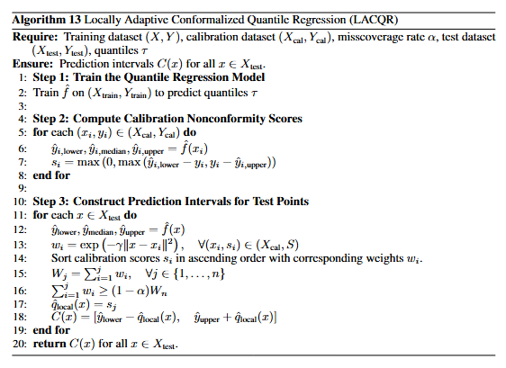
If we then test LACQR on the Diabetes test dataset, we can see how it performs. Based on the visualization of the predicted quantiles below, it can be seen that LACQR includes every data point within the quantiles. But, we can also see that the predicted intervals are very large in comparison to previous methods we have discussed.
For full performance, LACQR achieves a perfect final coverage of 100% when using \( \alpha=0.05 \). It also achieves an average interval width of 396.65 which is nearly double the size of CQR with the same hyperparameters. For those unaware, Gaussian kernels have a hyperparameter \( \gamma \) which controls the sensitivity of locality for the data points. A low \( \gamma \) means distant data points still contribute somewhat, and then the inverse for a high \( \gamma \). In this experiment, we use \( \gamma=1.0 \).
We can see how different values of \( \gamma \) affect performance. Using \( \gamma = 0.5 \) gets final coverage of 100% and average interval width of 404.87, \( \gamma = 1.0 \) gets final coverage of 100% and average interval width of 396.65, \( \gamma = 5.0 \) gets final coverage of 98.88% and average interval width of 356.97, and \( \gamma = 10.0 \) gets final coverage of 98.88% and average interval width of 352.51. So even with a focus on closer data points, LACQR produces very large interval widths.
To recap, LACQR extends CQR by computing an adaptive threshold for each test point based on the conformity scores of similar data points found in the calibration dataset.
Conformal Prediction for Time Series#
Now we will do a deep dive into conformal prediction for time series data. Just like both classification and regression methods, we will cover state-of-the-art algorithms, the maths, and the code behind each one.
Methods#
Unlike classification and regression, conformal prediction for time series methods is not split into Full and Split CP categories. This is due to the unique nature of sequential data.
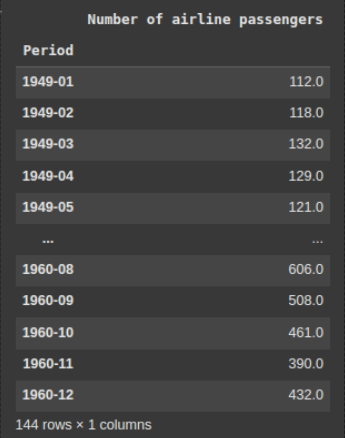
Alongside the maths and/or algorithms for each method, we will explore them through custom code implementations. In this section, we will use the Airline dataset to compare and empirically run the implementations. You can see a print of some entries of the dataset below.
For this task, we use a 1D convolutional quantile neural network to capture local temporal dependencies, the base performance can be seen below. It achieves a final coverage of 29.41% and an average interval width of 37.21. The Airline dataset is quite small, so achieving good coverage can be quite hard without more training data or advanced techniques.
See a zoomed-in version of the graph below, where the test data and predicted quantiles are more easily visualized.
Weighted Conformal Prediction for Distribution Drift#
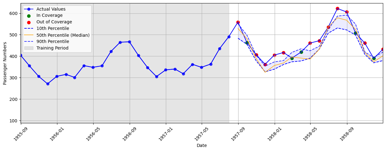
The first CP method for time series data we will explore is Weighted Conformal Prediction for Distributional Drift (WCP). As you have seen with the base model, time series add complexities, so WCP accounts for these in a handful of ways. The most notable is the concept of weighted thresholds.
The full Algorithm for WCP can be seen above. As always, the first step is the train the base model \( \hat{f} \) to predict the quantiles \( \tau \). The second step is the select the calibration dataset. Since in time series data the data distribution shifts over time, the calibration dataset is the most recent sample from the training dataset.
$$ X_{\text{cal}} = X_{\text{train}}[-n_{\text{cal}}:], \quad Y_{\text{cal}} = Y_{\text{train}}[-n_{\text{cal}}:] $$
This way allows the CP method to adapt to the most recent data distribution. Evidently, the larger \( n_{\text{cal}} \) is the more calibrated the method will be as it can observe longer-term trends. The third step is the compute exponentially decaying weights. Again, since the data distribution shifts over time, we want the older calibration data points to contribute but with a reduced influence. The fourth step is to compute the weighted threshold \( \hat{q} \), which uses the weights \( w \) to handle time-dependent drift. The final step is to construct the prediction intervals. This is done the same as regression CP methods.
You can see the code for WCP split up into the steps below. The second step selects the last \( n_{\text{cal}} \) data points from the training data set.
calibration_size = 50

calibration_data = y_train[-calibration_size:]
calibration_predictions = model.predict(x_train[-calibration_size:])

calibration_lower = calibration_predictions[:, 0]  # 10th percentile
calibration_median = calibration_predictions[:, 1]  # 50th percentile
calibration_upper = calibration_predictions[:, 2]  # 90th percentile

calibration_scores_lower = np.abs(calibration_lower - calibration_data.flatten())
calibration_scores_upper = np.abs(calibration_upper - calibration_data.flatten())
Then exponentially decaying weights can be calculated and normalized so WCP can prioritize more recent data points.
def calculate_weights(n, decay_factor=0.95):
    return np.array([decay_factor ** (n - i - 1) for i in range(n)])

weights = calculate_weights(len(calibration_scores_lower))
normalized_weights = weights / np.sum(weights)
Finally, for each test point, WCP computes the weighted thresholds \( \hat{q} \) using the calibration conformity scores \( s \) and the normalized weights \( w \). The upper and lower thresholds are then added and taken away from the upper and lower predicted quantiles from the model to construct the final prediction interval.
for i in range(len(x_test)):
test_prediction = model.predict(x_test[i].reshape(1, -1, 1), verbose=0).flatten()
test_lower = test_prediction[0]
test_upper = test_prediction[2]
qhat_lower = weighted_quantile(
calibration_scores_lower,
quantile=1 - alpha,
weights=normalized_weights
)
qhat_upper = weighted_quantile(
calibration_scores_upper,
quantile=1 - alpha,
weights=normalized_weights
)
lower_bound = test_lower - qhat_lower
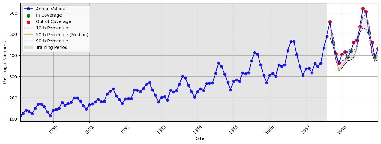
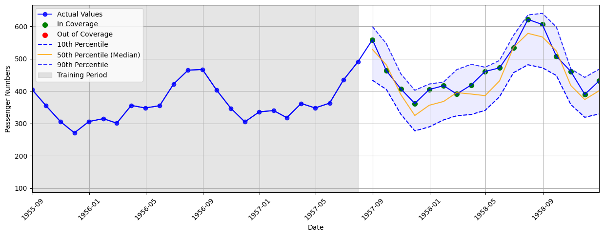
upper_bound = test_upper + qhat_upperIf we test WCP on the Airline dataset, we will be able to see how the base time series method performs! Based on the visualization of the calibrated quantiles below, we can see that WCP performs much better than the base neural network. All of the test points in the visualization are included within the calibrated quantiles which is perfect!
In terms of full performance, WCP achieves a perfect final coverage of 100% when using \( \alpha=0.05 \). It does this with an average interval width of 200.04. This is a great initial CP method for time series data!
To recap, WCP adapts CP for time series data by focusing on more recent data points than older ones. This allows it to adapt to distributional drift within the data.
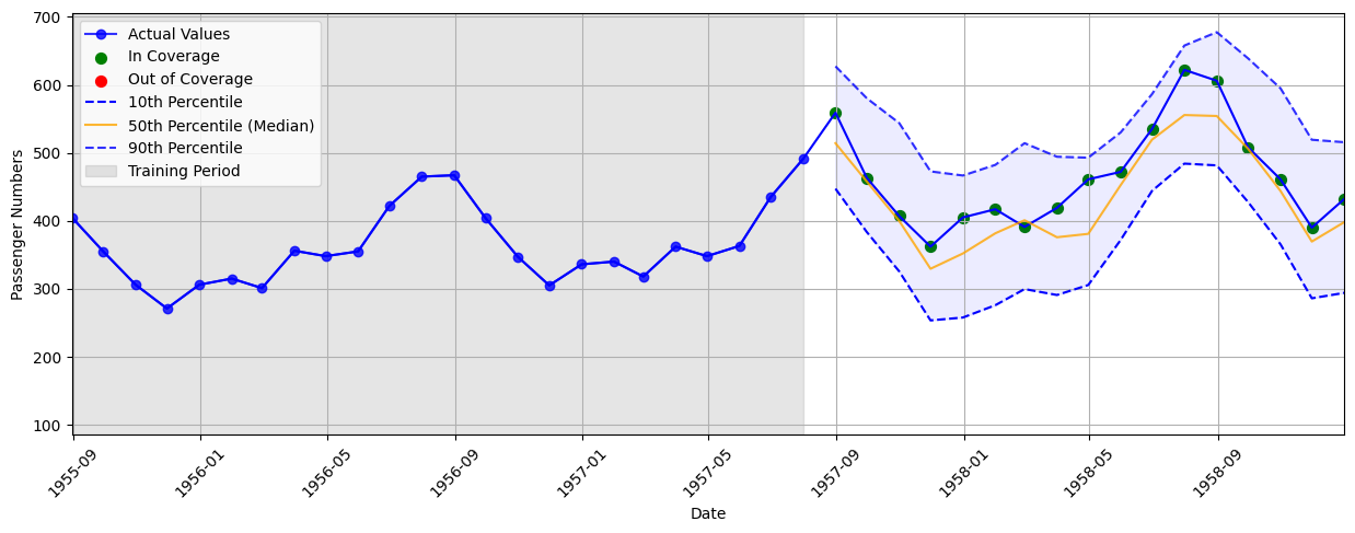
Adaptive Conformal Inference Under Distribution Shift#
As with the initial classification and regression CP methods, the thresholds \( \hat{q} \) produced are static for every test data point. Thus, the obvious extension is to introduce adaptive thresholds like in APS and LACQR. Adaptive Conformal Inference Under Distributional Shift (ACP) introduces these adaptive thresholds in a unique way for time series data.
The algorithm is ACP can be seen above. The only change from WCP is to step 4, the construct of the prediction intervals for all test points. Due to the nature of time series data, simply constructing a threshold \( \hat{q} \) for each test point is not viable. So to adapt it to time series, ACP first initializes a new misscoverage parameter \( \alpha_t = \alpha \) before any test points have been inferred upon. It then calculates the thresholds \( \hat{q} \) and constructs the prediction intervals as normal. This is where the adaptive part is added. Based on the last predicted interval, \( \varepsilon_t \) denotes if the prediction was in or out-of-coverage. Finally, \( \alpha_t \) gets updated using the error \( \varepsilon_t \) and the learning rate/step-size \( \gamma \). If the prediction was out-of-coverage, \( \alpha_t = \alpha_t + \gamma (\alpha - 1) \) essentially increases the misscoverage rate. This means for the next prediction, the thresholds \( \hat{q} \) will be looser to try and increase coverage. If the prediction was in-coverage, \( \alpha_t = \alpha_t + \gamma (\alpha - 0) \) essentially decreases the misscoverage rate. This means for the next prediction, the intervals will be tighter because \( \alpha_{t+1} > \alpha{t} \).
You can see the altered prediction set creation in the code below. Remember to check out my GitHub Repo!
alpha_t = alpha

for i in range(len(x_test)):
    test_prediction = model.predict(x_test[i].reshape(1, -1, 1), verbose=0).flatten()

    test_lower = test_prediction[0]
    test_upper = test_prediction[2]

    qhat_lower = weighted_quantile(
        calibration_scores_lower,
        quantile=1 - alpha_t,
        weights=normalized_weights
    )
    qhat_upper = weighted_quantile(
        calibration_scores_upper,
        quantile=1 - alpha_t,
        weights=normalized_weights
    )

    lower_bound = test_lower - qhat_lower
    upper_bound = test_upper + qhat_upper

    actual_value = y_test[i]
    if lower_bound <= actual_value <= upper_bound:
        err_t = 0  # In coverage
    else:
        err_t = 1  # Out of coverage

    alpha_t = alpha_t + gamma * (alpha - err_t)
The key addition is the conditional \( \varepsilon_t \) variable that is used to increase or decrease the misscoverage rate \( \alpha_t \) dynamically.
If we test ACP on the Airline dataset, we will be able to see how these adaptive thresholds improve performance. Based on the visualization of the calibrated quantiles below, we can see that ACP includes all data points within the predicted quantiles but with tighter intervals than WCP.
In terms of full performance, ACP achieves a perfect final coverage of 100% when using \( \alpha=0.05 \). It does this with an average interval width of 135.94. This is much lower than WCP which had the same coverage and an average width of 200.04.
To recap, ACP adds adaptive thresholds to WCP by decreasing the misscoverage rate \( \alpha \) for successive in-coverage predictions as well as increasing it for successive out-of-coverage predictions. This of course assumes access to ground truth labels/feedback calculate \( \varepsilon_t \).
Risk-aware Conformal Prediction#
Now we will do a deep dive into risk-aware conformal prediction. Like previous classification and regression methods, we will cover relevant methods, the maths, and the code behind each one.
Methods#
Risk-aware CP is conformal prediction that incorporates risk-awareness, this is particularly useful for safety-critical scenarios such as autonomous driving- misclassifying a pedestrian is probably worse than misclassifying a traffic cone. Therefore, incorporating risk-awareness into existing CP methods would be beneficial.
Alongside the maths and/or algorithms for this method, we will explore it through custom code implementations. In this section, we will go back to the MNIST digits dataset. You can see a print of some images from the dataset below.
Risk-aware CP#
Risk-aware CP adapts Split CP for Classification by assigning different weights to classes based on false positive (FP) and false negative (FN) costs. This is crucial in scenarios where misclassification impacts are not equal. In many real-world applications, FPs and FNs have asymmetric consequences. For example, in medical diagnosis, FN is worse as missing a positive case could mean no treatment, leading to severe consequences.
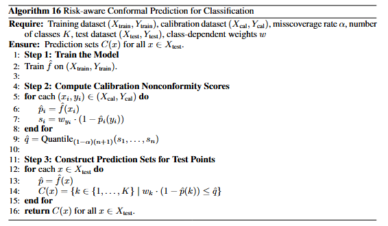
The algorithm for Risk-aware Split CP for classification can be seen above. It is pretty much the same as Split Inductive CP except for three key additions/alterations. The first is the requirement for a set of class-dependent weights \( w \), a scalar value for each class \( k \in K \). If \( w_k < 1 \), it means we have assigned a higher weight to avoid false negatives for class \( k \). Whilst \( w_k > 1 \), it means we have assigned a higher weight to avoid false positives for class \( k \).
The second change is in step 2 of the algorithm, where the conformity scores are computed for the calibration dataset. The method multiplies the conformity score \( 1-\hat{p}_i(y_i) \) by the corresponding class-dependent weight \( w_{y_{i}} \). Previously, each class was treated equally, with nonconformity only depending on the probability of the correct class. Caring about FNs (\( w_k < 1 \)) means that the class \( k \)’s conformity scores will be lowered, making the threshold later looser for that class, thus, avoiding false negatives. Focusing on FPs (\( w_k > 1 \)) means that the class \( k \)’s conformity scores will be inflated, making the threshold later stricter for that class, thus, avoiding false positives.
The final change is for step 3 when the prediction sets are constructed. Typically, the prediction set was based only on class probabilities. Now, it scales the confidence threshold by the class risk weight \( w_k \).
You can see the code for Risk-aware Split CP below. Remember to check out my GitHub Repo!
weights = np.ones(10)  # Initialize weights for all classes
weights[1] = 0.5         # Set higher weight for digit '1'

cal_probs = model.predict(x_cal)

cal_scores = []
for i in range(len(y_cal)):
    true_label = np.argmax(y_cal[i])
    true_prob = cal_probs[i, true_label]
    score = weights[true_label] * (1 - true_prob)  # Cost-sensitive nonconformity score
    cal_scores.append(score)
cal_scores = np.array(cal_scores)
We define the base weights as all ones to start. Having all weights equal to 1 is equivalent to Split CP with no risk-awareness. Weights can then be specifically assigned depending on what is wanted. Then in the calibration step, the conformity scores are weighted by the corresponding true label’s weight.
for i in range(len(test_probs)):
    prob_vector = test_probs[i]
    true_label = np.argmax(y_test[i])

    prediction_set = []
    for label in range(10):
        score = weights[label] * (1 - prob_vector[label])
        if score <= q_hat:
            prediction_set.append(label)
Finally, the conformity score at inference time is also multiplied by the corresponding true label’s weight.
If we test Risk-aware Split CP on the MNIST digits dataset, we will be able to see how it adapts to different weights. First, we test the base Split CP’s (\( w = 1 \)) abilities and visualize some predictions below. This will serve as our baseline. The base CP method has a top-1 accuracy of 97% and a coverage of 98%.
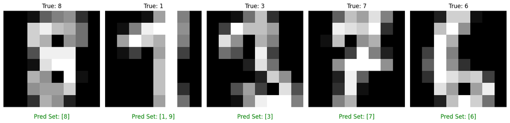
We can then change \( w_{1} = 2 \), making Risk-aware Split CP care about false positives for class 1. Below is the visualization of some predictions. It is clear that this forces the threshold for 1 to be a lot higher, and in this case, become too conservative and remove the correct label from the second image. This has a coverage of 95% as a result.
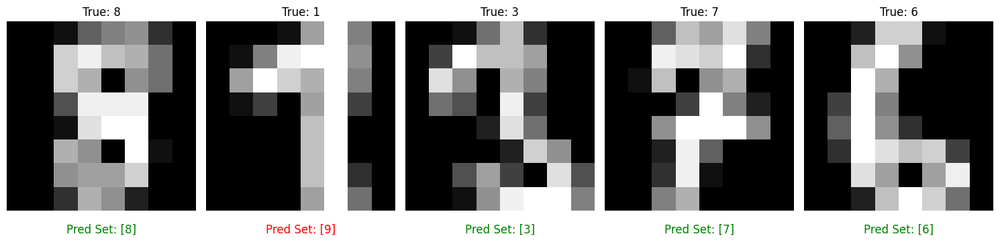
To recap, Risk-aware Split CP assigns different weights to classes to force the method to care more about false positives or false negatives. This makes it ideal in safety-critical scenarios such as healthcare.
Applicative Considerations#
Conformal Prediction is a powerful framework for uncertainty quantification, but its effectiveness in real-world applications depends on various considerations, including data properties, computational constraints, and the choice of method. One of the most critical aspects is whether the data satisfies the exchangeability assumption. Standard CP methods rely on the assumption that the training, calibration, and test data come from the same underlying distribution. When this assumption holds, CP provides reliable prediction sets with guaranteed coverage. However, in applications where data distribution shifts over time, such as financial forecasting, standard CP can become less reliable. In such cases, techniques like Weighted Conformal Prediction or Locally Adaptive CP help account for distributional drift by prioritizing recent calibration samples over older ones.
The choice between full and split conformal prediction also impacts practical deployment. Full CP provides finite-sample validity but is computationally expensive, as it requires retraining the model for each test point. This makes it impractical for large-scale real-time applications, such as fraud detection or high-frequency trading. Split CP, on the other hand, is computationally efficient but sacrifices some statistical efficiency due to reduced calibration data. Applications with strict real-time constraints often favour Split CP or variants like Cross-Conformal Prediction, which balance computational cost and coverage guarantees.
Task-specific modifications of CP further refine its applicability. In classification, Risk-Aware CP allows users to assign different importance levels to classes, ensuring that high-risk misclassifications, such as in medical diagnostics or autonomous driving, receive stricter coverage constraints. In regression, Conformalized Quantile Regression (CQR) extends CP to asymmetric prediction intervals, which is particularly useful in fields like meteorology and energy forecasting, where uncertainty is often skewed.
Beyond technical considerations, the interpretability of CP is crucial for deployment in sensitive domains. Unlike standard deep learning confidence scores, CP provides well-calibrated uncertainty estimates, which are easier to communicate to stakeholders in healthcare, finance, and law enforcement. However, the size of prediction sets must be carefully managed to balance informativeness and usability. Overly large sets may ensure coverage but become impractical for decision-making, while overly small sets risk excluding the true label. Adaptive CP methods address this by dynamically adjusting intervals based on the difficulty of the prediction.
The Future of CP#
Conformal Prediction has already established itself as a valuable framework for uncertainty quantification, offering valid and reliable prediction sets across a wide range of applications. Come on, just look at how many A* conferences/journals most of the papers are in each year! One of the most promising directions is the integration of CP with deep learning and foundation models. Traditional CP methods are often computationally demanding when applied to large-scale neural networks, but recent advances in approximate full conformal techniques aim to bridge this gap, making CP more practical for deep learning applications such as generative AI, large language models, and high-dimensional computer vision tasks.
Split CP methods can be used instead as they are computationally efficient because they use a holdout set instead of retraining the model. Recent advances in Split methods have attempted to increase coverage (due to looser guarantees than FCP methods) whilst lowering the average set size. Other advancements could also look towards reducing the size/quality of the calibration dataset to reduce how much extra data is needed to achieve decent coverage guarantees.
Fairness and robustness are also key considerations in the future of CP. As machine learning systems increasingly influence high-stakes decisions in areas like healthcare, criminal justice, and hiring, it is critical to ensure that conformal methods do not reinforce existing biases. Risk-aware CP, which allows for differential weighting of predictions based on real-world costs, is an important step toward making CP more aligned with ethical and safety considerations. Additionally, robust CP methods that account for adversarial attacks or worst-case scenarios are being explored to enhance reliability in security-critical applications.
Helpful Resources#
I have curated some other helpful CP resources for you to have a look through, and continue your CP journey:
- A Gentle Introduction to Conformal Prediction and Distribution-Free Uncertainty Quantification. This paper breaks down a few CP methods, as well as some history behind CP. It is by Anastasios Angelopoulos, an important researcher in UQ and CP.
- Awesome Conformal Prediction. This is a large and active GitHub Repo that announces new CP papers and tutorials.
- MAPIE. An open-source Python library that applies basic conformal prediction wrappers over models. Useful when you want CP quickly but only basic versions of methods.
- Conformal Prediction: A Visual Introduction. This is a very handy visualization of how CP works. It is pretty short, but very fun to mess around with.
GitHub Repo#
Implementation and tutorial for dozens of Conformal Prediction Algorithms across classification, regression, time-series, and risk-aware tasks.
Conclusion#
This tutorial introduced you to conformal prediction (CP)- a framework designed to provide reliable uncertainty quantification. I hope you now have a deeper understanding of how CP works in many different modalities, including an understanding of the intuitive maths and code I provided.
The blog post + maths + code has taken me a few months to create for you. This now currently serves as the largest CP tutorial on the internet! If this has helped you out in anyway, please let me know in the comments below! 😄