Demystifying Kolmogorov-Arnold Networks: A Beginner-Friendly Guide with Code

Introduction

#

Kolmogorov-Arnold Networks (KANs) [1], inspired by the Kolmogorov-Arnold representation theorem [2], are promising alternative to neural networks (NNs). Coming out of MIT, KANs have been making waves everywhere you look, from Twitter to forums. The authors have some strong claims and it seems like everyone has boarded the hype train, but do they live up to the claims made? What are they and how do they work? Well, I will answer all of the following in this post and hopefully demystify some of the horrible jargon and notation that comes with them 🙂.

Kolmogorov-Arnold Networks (KANs)

#

Kolmogorov-Arnold Networks (KANs) are a new type of neural network (NN) which focus on the Kolmogorov-Arnold representation theorem instead of the typical universal approximation theorem found in NNs. Simply, NNs have static activation function on their nodes. But KANs have learnable activation functions on their edges between nodes. This section will delve deeper into the KAN architecture and then main differences between KANs and NNs, but first we need to discuss two concepts: the Kolmogorov-Arnold representation theorem and b-splines.

Kolmogorov-Arnold Representation Theorem

#

As stated earlier, KANs use the Kolmogorov-Arnold representation theorem. According to this theorem, any multivariate function \(f\) can be expressed as a finite composition of continuous functions of a single variable, combined with the binary operation of addition. But let’s step away from the math for a moment. What does this really mean if you’re not a mathematician?

Let’s imagine I asked you to make me some Baklava, a dessert with multiple ingredients and steps. At first glance, making Baklava might seem complex. However, the Kolmogorov-Arnold representation theorem suggests that any complex ‘recipe’ can be simplified into basic, one-ingredient recipes that are then combined in specific ways. Below is a visual breakdown of this process:

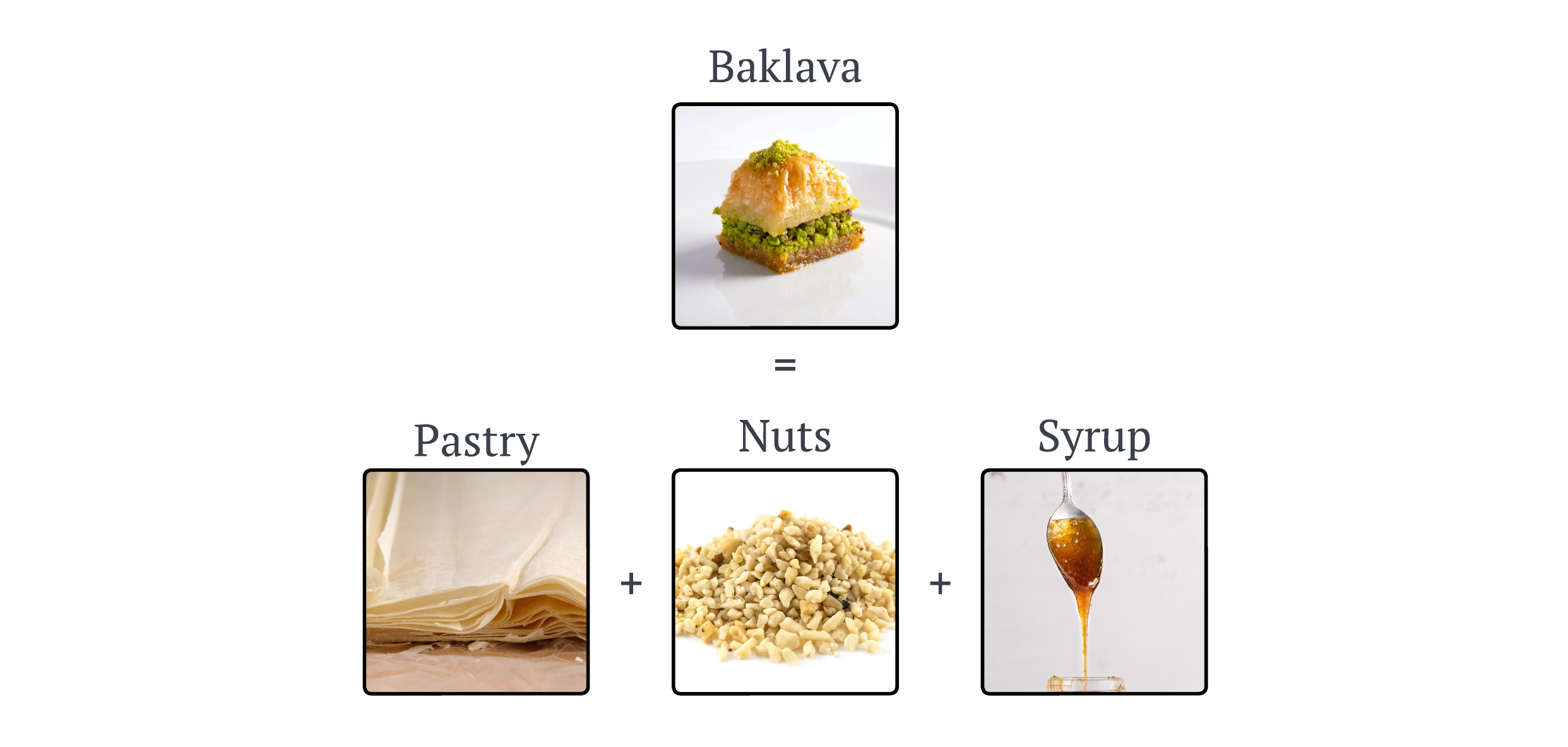
This image shows how the complex process of making Baklava can be broken down into simpler tasks like ‘chop the nuts’ or ’layer the pastry’. Each of these tasks handles one aspect of the recipe, akin to handling one variable at a time in a mathematical function. Bringing this back to the math, the theorem can be expressed as follows:

$$ f(x_{1},…,x_{n}) = \sum_{q=1}^{2n+1}\Phi_{q}(\sum_{p=1}^{n}\phi_{q,p}(x_{p})) $$

where \(f(x_{1},…,x_{n})\) is our multivariate function (complex recipe), \(\phi_{q,p}(x_{p})\) are the univariate functions (simple, one-ingredient recipes), and \(\Phi_{q}\) takes the univariate functions and combines them. By understanding this breakdown, we see how complex problems (or recipes) can be tackled one piece at a time, making the whole process more manageable.

B-splines

#

Formally, b-splines [3] are a sophisticated curve-fitting method and a specific type of spline [4] - a mathematical term for a flexible, piecewise-polynomial function that defines a smooth curve through a series of points. Informally, imagine you’ve plotted dots on a graph to represent how your spending has fluctuated over the past 10 months, and now you want a smooth line that best shows trends over those months. To do so we could use a polynomial fit, so let’s see how that might look.

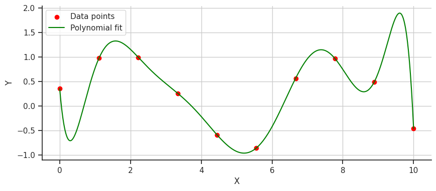
It works! We have a smooth line that shows my wild spending habits over the last 10 months. But if we look closer, specifically after the first data point, why does the line drop so drastically instead of just curving upwards towards the second data point? This issue with polynomial fitting is due to their tendency to exhibit wild oscillations, a problem known as Runge’s phenomenon.

How can we fit this line better…let’s try splines! A spline divides the data into segments and fits individual polynomials to each. Let’s see what a spline fit looks like.

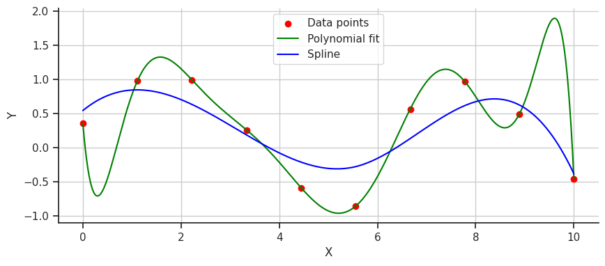
This fit is much smoother, but perhaps it’s a bit too gentle and underfits the data. This is where B-splines can step in to fix things. B-splines, a type of spline that uses control points to pull the curve and guide the polynomials to fit better, offer a more precise solution. Let’s take a look at a B-spline fit on the data.

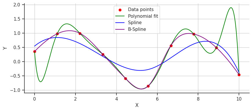
Perfect! The B-spline doesn’t oscillate wildly or underfit; instead, it captures the data perfectly. B-splines provide superior smoothness and crucial accuracy for modeling complex functions. They can adapt easily to changes in data patterns without requiring a complete overhaul of the model, making them a versatile and robust tool for data fitting.

Mathematically, we can define a b-spline as:

$$ C(t) = \sum_{i=0}^{n}P_{i}N_{i,k}(t) $$

where \(P_{i}\) are the control points, \(N_{i,k}(t)\) are the basis functions, and \(t\) is the knot vector.

KAN Architecture

#

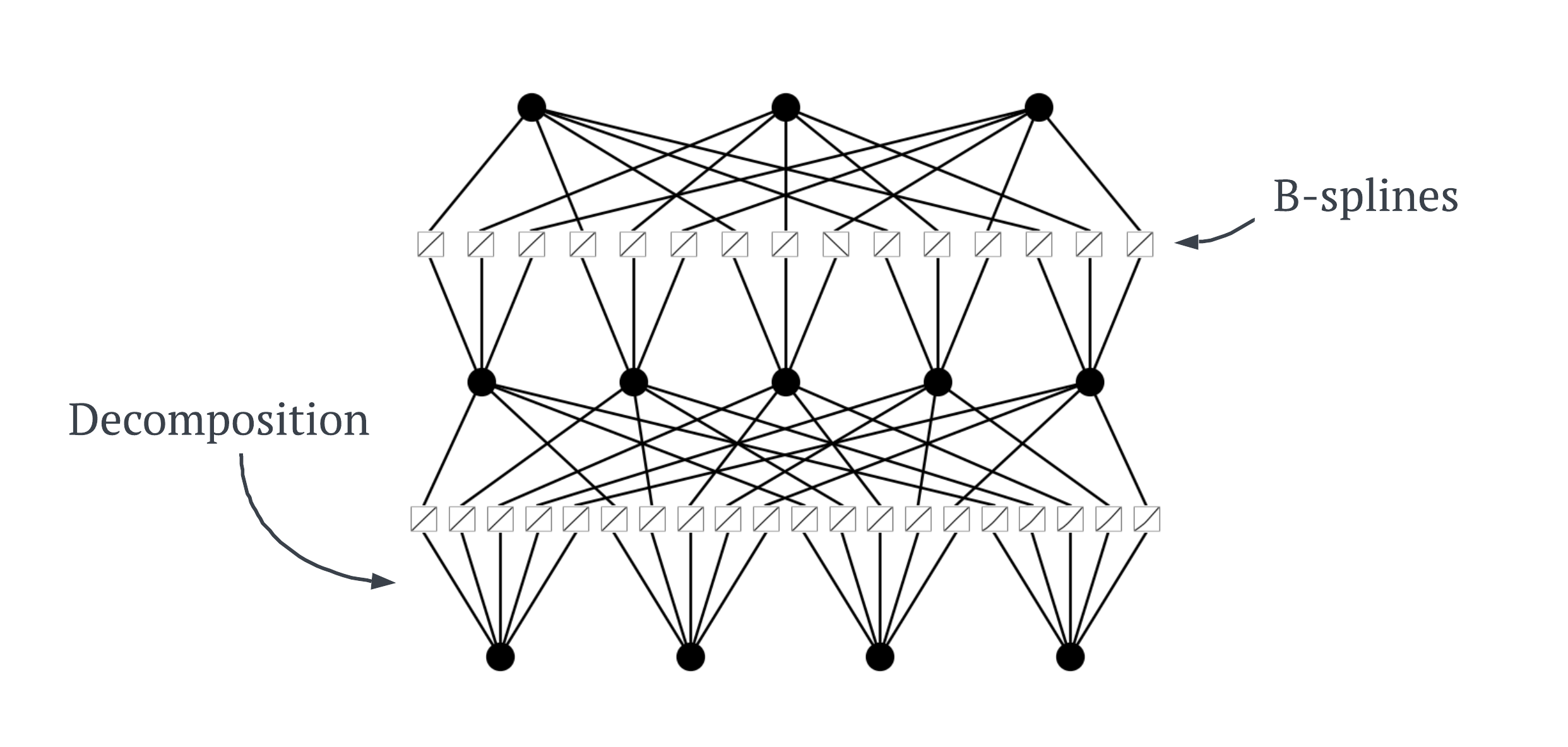
KANs represent a breakthrough in neural network design by leveraging the Kolmogorov-Arnold Representation (KAR) theorem alongside B-splines, creating a dynamic and powerful model. The KAR theorem shows us a way to decompose complex functions into simpler ones. KANs apply this principle at every edge within the network, making each edge between neurons a learnable B-spline activation function. This allows each edge to accurately learn its specific part of the data input much like making a specific part of a Baklava recipe. The KAN architecture can be seen below.

As KANs undergo training, the real excitement begins. Each B-spline adjusts its control points \(P_{i}\) through a process known as backpropagation, which is common in training neural networks but takes on a new dimension here. This adaptive process allows KANs to refine their approach to data with each training iteration, continuously improving their accuracy and efficiency.

Now that you understand how KANs are structured and adapt during training, let’s dive into a practical example. In the following sections, we’ll explore how to set up and train a KAN, using real data to see firsthand how these networks learn and evolve.

Creating and Training a KAN

#

To construct and train a KAN, first we can use the pykan package provided by the authors of the original KAN paper. We can install it locally using:

pip install pykan

For the remainder of this notebook, I will be testing KANs on the Iris toy dataset. You can see the full code for loading and preprocessing this dataset in my codebase!

We can construct a KAN with four inputs, 3 outputs, and 5 nodes in a single hidden layer by:

model = KAN(width=[4, 5, 3], grid=5, k=3)

I use a 3rd order spline and 5 grid intervals as my params. We won’t go into too much detail about these in this post. Let’s see what this looks like.

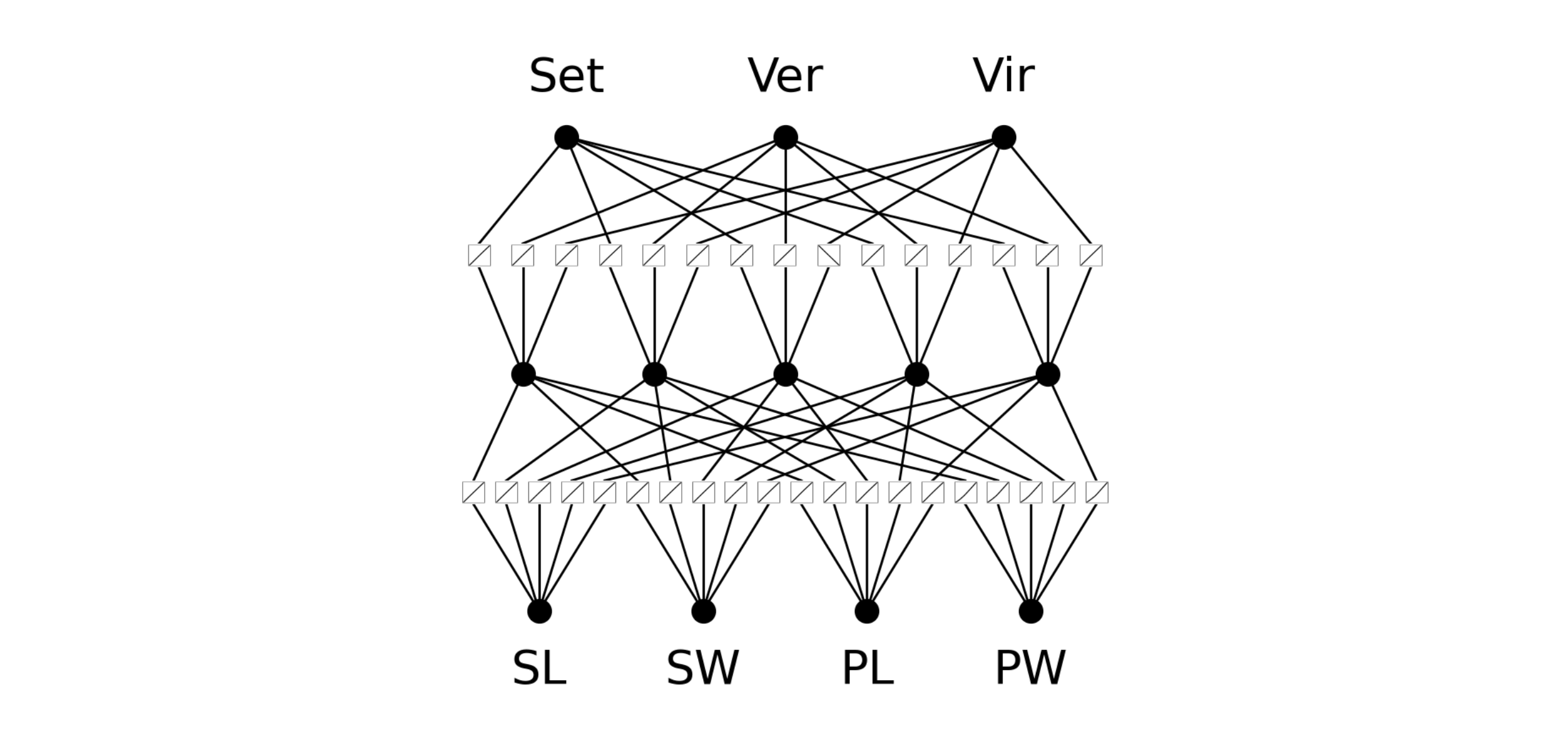
Cool! So we have a small KAN and we can see all of the initialized b-splines on the edges between neurons. In this example, the bottom four variables represent our inputs for the Iris dataset (sepal length, sepal width, petal length, and petal width) and the top three are the three different types of irises’ we are trying to predict.

So, now let’s train this KAN. We can do this very similarly to a standard neural network using an optimizer, a loss function, a number of epochs, and uniquely, penalty parameters which we will not put much detail into in this blog post.

results = model.fit(iris_dataset, opt="Adam",
                    metrics=(train_acc, test_acc),
                    loss_fn=torch.nn.CrossEntropyLoss(),
                    steps=100, lamb=0.01, lamb_entropy=10)

We will use Adam as the optimizer, CrossEntropyLoss as our loss function (since we are doing multiclass classification), and 100 epochs. This takes 8.5 minutes to train and we get a train and test accuracy of (0.992, 0.934) respectively. We can both agree this was clearly successful! Take a look at how our b-splines morphed during training.

In the initial set of epochs, our b-splines change shape a lot until eventually converging into a stable shape. Let’s see what our KAN looks like now.

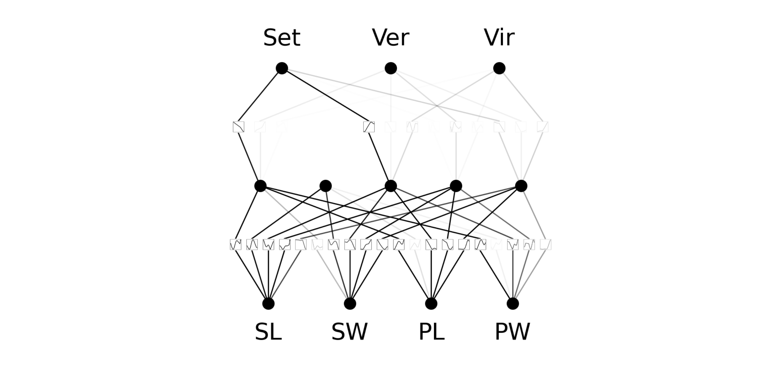
This is interesting, some of the edges have disappeared completely?! I won’t go into full details, as it is unnecessary, but neurons that have activity below a certain threshold are fully switched off to make the network more efficient. We can actually prune this network to make to no completely remove the inactive nodes. The code below will very simply do this for you.

model = model.prune()

Once again, let’s see what our KAN looks like now.

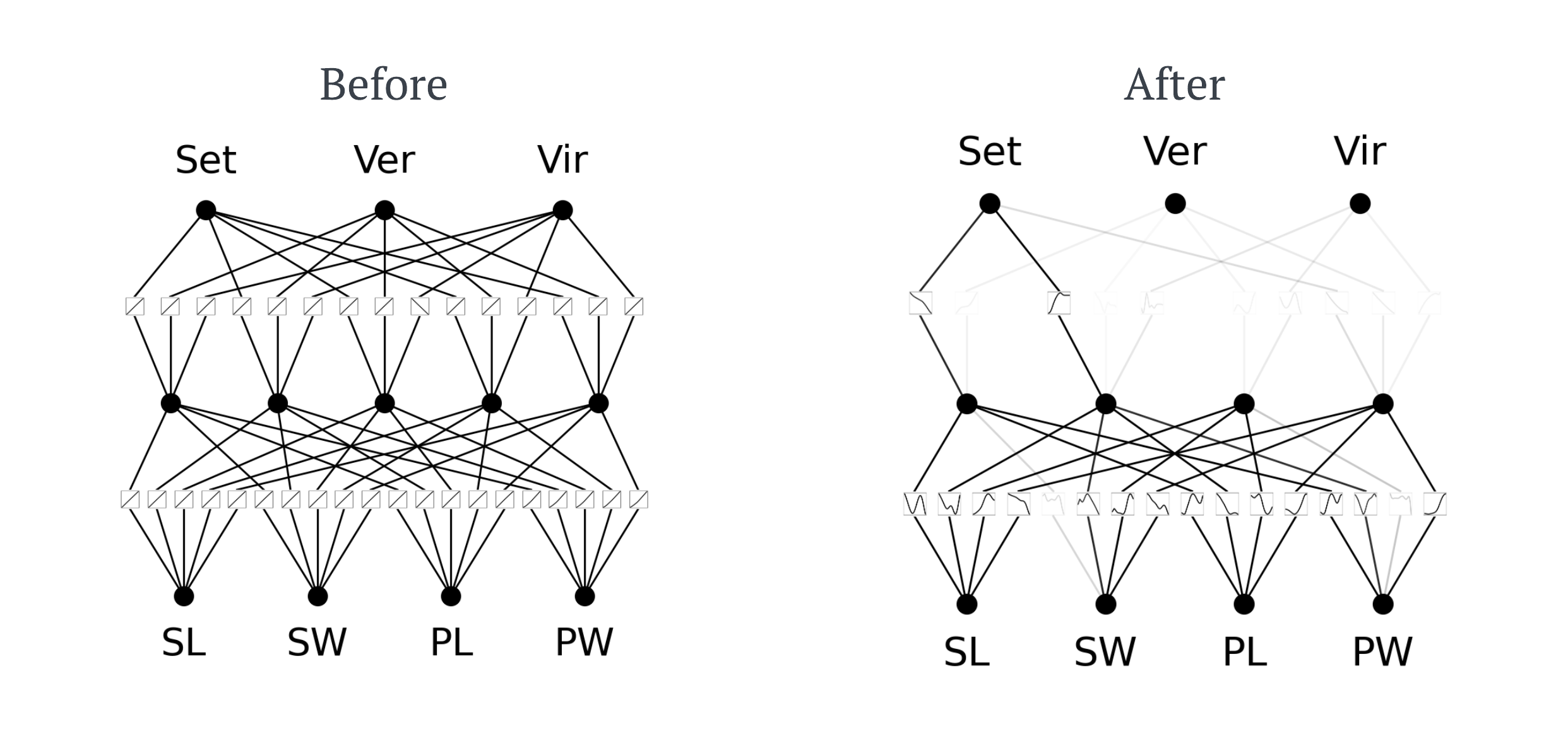
As you can see, the hidden layer of 5 nodes has been pruned down to 4 making the KAN more computationally efficient without reducing accuracy. We can now fine-tune this KAN again, only 50 epochs this time, and achieve a train and test accuracy of (1.0, 1.0) respectively.

We have now constructed, trained, pruned, and fine-tuned a KAN. We did all of this with some simple code too! Even though this is a small network, it shows how powerful KANs can actually be. Before we see how they compare to traditional neural networks, I want to show you the best feature of KANs.

We can now extract the symbolic formula of the network. This makes more sense if I just show you. For instance, take the first class (Setosa) that we are trying to predict. The symbolic formula that the KAN has learnt for this class is:

$$ 1.61(-\sin(0.55x_{3} + 9.34) + 0.12\tan(0.57x_{1}\cdots $$

We can do a lot with this formula. But if we take the formula for the whole network, inference can be done on that instead of the network meaning once again we save a lot of computation. Since it is the same formula that the network uses, we don’t lose any accuracy by inferring on this instead of the network. Isn’t that cool!

Comparison to Neural Networks

#

The authors behind KANs have made some…wild…claims regarding them in comparison to neural networks (if you are interested, just look towards Twitter). So, let’s do a little experiment ourself to see how they compare. Firstly, we will create a neural network with the same architecture.

self.fc1 = nn.Linear(4, 5)
self.relu = nn.ReLU()
self.fc2 = nn.Linear(5, 3)

We will train this network on the Iris dataset using the same optimizer, loss function, and number of epochs as we used on the KAN. The table below show the results between the two models.

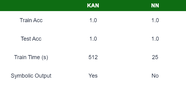
Both models can achieve a high accuracy, well actually a perfect accuracy. A major comparison is training time, the neural network only requires a fraction of the training time needed. These tests were only performed on tiny architectures. When I increase the size of the KAN, training time starts to take ~30 mins on my expensive GPU. However, the KAN can provide symbolic formulas for the learnt splines, particular output nodes, and the network as a whole.

When I trained both models on the California Housing regression dataset, I obtained the following results.

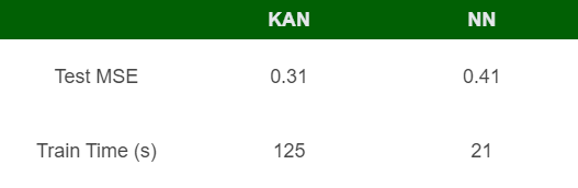
Beyond toy datasets, it is possible that the KAN architecture could be more accurate than the standard dense neural network. However, the training time to achieve the improved performance is poor. If we trained the neural network for the remaining ~100s difference, we could probably see similar or better results bar a symbolic output.

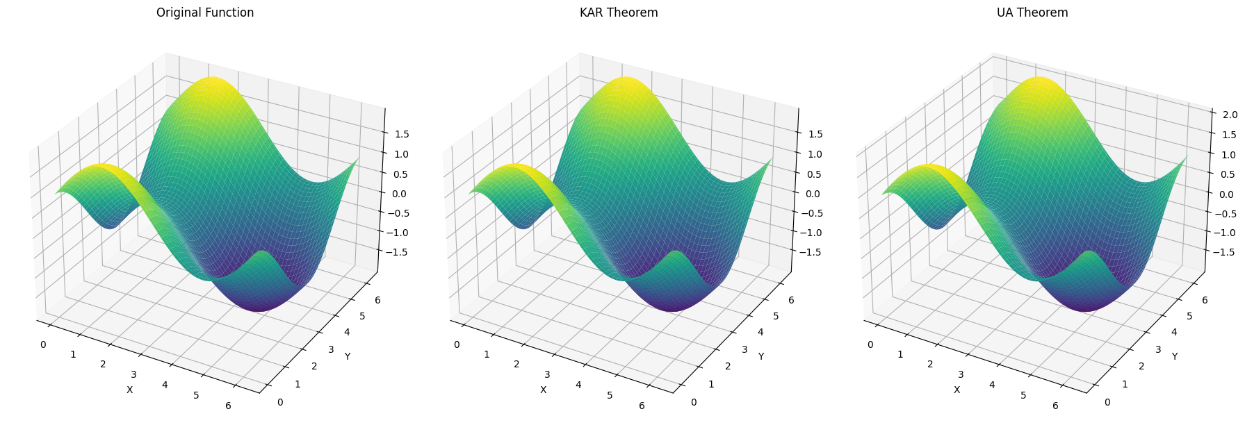
Just for an excuse to make a fun plot, below is a KAN and NN’s attempt to approximate the function for the sum of sine x and cosine y. They both achieve 100% accuracy, but I thought this would be fun to see how they both can successfully perform the same task but using two different methods. Plus, I couldn’t waste a good image 😄.

So Why KANs?

#

So far we have seen that KANs can reach better accuracy than MLPs (in some cases), and output a symbolic formula, but at the cost of incredibly slow training. So why would you use a KAN over an MLP? Here are my thoughts on applications:

• Mobile applications. Predictive networks have a hard time trying to balance high accuracy and low compute, due to low computational resources on phone. I feel like KANs would excel here as they can achieve a high level of accuracy, then we get convert the network into a symbolic formula. Evidently, inference can be done on this formula and not the expensive network.
• Science-related tasks. An science-related task, such as fitting physical equations or PDE solving, would be ideal.
• Interpretability. In rare cases where interpretability is a main focus over other factors, a KAN would be ideal or current interpretability methods in MLPs, such as SHAP, or LIME values.

Currently, I personally feel like uses cases are limited. If certain limitations of KANs, such as slow training speed and instability, can be mitigated then they would have a lot more applications.

Conclusion

#

Kolmogorov-Arnold Networks present a unique alternative to traditional neural networks. In this blog post our exploration has revealed that while KANs have the potential to reach higher accuracy and offer unique advantages such as symbolic representation of learned functions, they come with significant trade-offs. The most notable among these is the long training time, which can be a major factor for practical applications. Despite this, KANs offer exciting prospects for future research and development.

I hope that this blog post made KANs easier to understand, and that the code I have provided will allow you to mess around with them yourself. I am planning on explore KANs myself much further and I will constantly post further blog posts regarding my experiments.

References

#

[1] Liu, Z., Wang, Y., Vaidya, S., Ruehle, F., Halverson, J., Soljačić, M., Hou, T.Y. and Tegmark, M., 2024. Kan: Kolmogorov-arnold networks.

[2] Akashi, S., 2001. Application of ϵ-entropy theory to Kolmogorov—Arnold representation theorem. Reports on Mathematical Physics, 48(1-2), pp.19-26.

[3] De Boor, C., 1972. On calculating with B-splines. Journal of Approximation theory, 6(1), pp.50-62.

[4] Ahlberg, J.H., Nilson, E.N. and Walsh, J.L., 2016. The Theory of Splines and Their Applications: Mathematics in Science and Engineering: A Series of Monographs and Textbooks, Vol. 38 (Vol. 38). Elsevier.

Codebase

#