Robust Uncertainty Quantification using Conformalised Monte Carlo Prediction

Introduction

#

Recently, I attended AAAI ‘24 to present a paper that got accepted titled “Robust Uncertainty Quantification using Conformalised Monte Carlo Prediction”. In this blog post I will walk you through the paper in a more informal manner and how our method, MC-CP works. Take a look at any of the links above before you read the rest of this post.

MC-CP is a conformal prediction algorithm that produces sets/intervals of smaller size without any reduction in prediction performance. So as a nice easy walkthrough I will cover a brief introduction into conformal prediction, the MC-CP method, our results, and finally where future work could look towards. I encourage you to check out our GitHub implementation also!

Motivation

#

Firstly, this may be the first time that some of you are hearing the words ‘Conformal Prediction’, so let’s run through this concept. Conformal Prediction [1] is an inference time technique that, put simply, generates prediction sets/intervals instead of singletons for any given model. The sets/intervals are generated with a confidence level. The larger the set/interval, the more unsure the model is about its prediction, whilst a narrow set/interval signifies confidence.

But why would we want that? The simple answer to that it to look at the image below. Here we have an MRI scan of a random person’s brain. If we trained a neural network on images similar to these and its task was to predict if any diseases are present, it might predict that this image shows a biomarker for Multiple Sclerosis. Now if a doctor had 100% trust in their AI models (hopefully they don’t 😅), they would start providing treatment for this disease. But as we know the majority of biomarkers are not unique to one disease, and AI model are not 100% accurate, so if the patient did not have Multiple Sclerosis, then more harm would come to them than good.

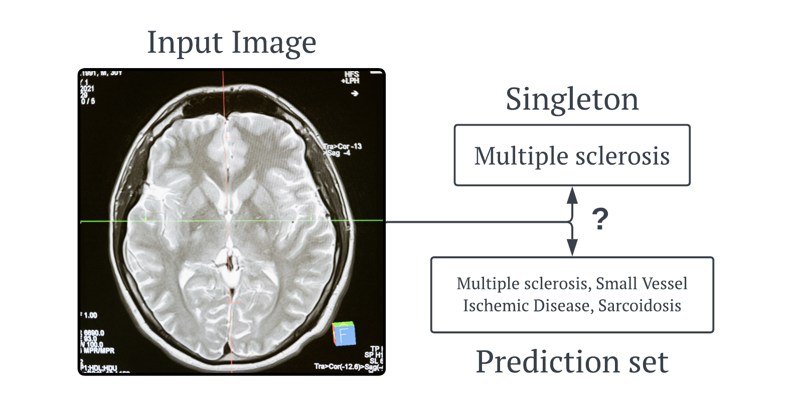
So if the doctors AI model uses conformal prediction, it would give them a set of diseases. In the image above, all the diseases in the set have this same biomarker. Now the doctor can make an informed decision about the possible treatment to give the patient.

But what if the model is 99% accurate, why would we need this? As we all know, it is very rare/difficult to get a model to predict such high prediction performance and in all tasks there will be that 1% that the model gets wrong or is very unsure about. This is where conformal prediction is at it’s strongest, it is a really simple way to understand the model’s confidence/uncertainty in its prediction. Yes, you could develop some fancy uncertainty quantification method that gives a salient estimate. But to a doctor/any other user, this number means nothing to them but a prediction set/interval does. They can look at the size and quickly understand that the model was either confident or uncertain.

So why have we developed a new conformal prediction algorithm if they are so good? Current state-of-the-art conformal prediction algorithms have a tendency to overestimate [2], meaning they produce larger set/interval sizes than necessary. And this is specifically where out motivation lies, we wanted to create a new conformal prediction algorithm that reduces this set/interval size.

MC-CP

#

Monte-Carlo Conformal Prediction (MC-CP) is comprised of two parts: a new Adaptive Monte-Carlo Dropout, and a conformal prediction algorithm. You can see a high-level overview of this method in the image below. In these sections below I will go over the Adaptive Monte-Carlo Dropout method and MC-CP for image classification.

Adaptive Monte-Carlo Dropout

#

As a little refresher, Monte-Carlo Dropout [3] is an inference time technique that executes multiple forward passes of each input data through the deep learning model. Dropout layers that are typically turned off during inference are kept on during this process. What you get is a variational approximation to epistemic uncertainty within the model. Or in simpler terms, Monte-Carlo Dropout is a method where a deep learning model keeps randomly turning off parts of itself during predictions, not just during training. This process allows the model to make multiple guesses for each data point, helping to measure how confident it is about its predictions.

As you can expect, running model the model for \(\mathbb{N}\) forward passes for each test data point can be computationally demanding. We wanted to reduce this computational demand without sacrificing uncertianty estimates, and our solution was found in the Law of Large Numbers [4].

Each forward pass with MC Dropout can correspond to a particular model instantiation. Therefore, MC Dropout can be modelled as a Bernoulli process. Some of these model instantiations adds unique variance to the prediction distribution whilst some produce similar or the exact same predictions. Hence, whilst the prediction variance may be large during the first few forward passes, as we go on this variance value becomes smaller due to the Law of Large Numbers. At the point where new predictions stop adding much variance then we could stop MC Dropout early to save computation as remaining forward passes add little to no value. And so we created Adaptive MC Dropout, which you can see the python code for below!

def adaptive_mc(model, x_train, y_train, x_test, y_test, output_dims):
    patience, min_delta, max_mc = 10, 5e-4, 1000
    montecarlo_predictions, var_diffs = [], []
    for image in tqdm.tqdm(x_test):
        predictions, prev_variance, current_patience_count = [], [], 0
        while len(predictions) < max_mc:
            prediction = model.predict(np.expand_dims(image, axis=0), verbose=0)
            predictions.append(prediction)
            variance = np.array(predictions).std(axis=0)
            if predictions[1:]:
                var_diff = abs(prev_variance - variance)
                var_diffs.append(var_diff)
                current_patience_count = current_patience_count + 1 if np.all(var_diff <= min_delta) else 0
            if current_patience_count > patience:
                break
            prev_variance = variance
        montecarlo_predictions.append(np.mean(predictions, axis=0))
    return var_diffs

Adaptive MC Dropout takes two parameters: the threshold \(\delta\) and the patience counter \(P\). If you are familiar with early stopping in deep learning then this piece of code will be easy to follow. In essence, during the MC Dropout process, we track the variance overtime. We then calculate the absolute difference between the previous forward passes variance and the current forward passes variance. If this difference in below the threshold \(\delta\), then a counter is incremented. Once all classes/quantiles converge below \(\delta\) for \(P\) consecutive forward passes, then we declare the MC Dropout process converged and stop it early.

This plot below shows and example of the difference in variance overtime for an example image input where \(\delta = 4e-5\), \(P = 10\) and the maximum forward passes is \(1000\). As you can see variance in high towards the left of the plot but as the number of forward passes increases, this slowly reduces. At forward pass \(245\), all classes fall below \(\delta\) and \(P\) forward passes later all classes are still below the threshold and it stops early. In comparison to traditional MC Dropout, we save \(\approx 75\)% of computation on this input alone. Of course, over a whole test dataset in in deployment this can add up to be a lot.

MC-CP for Image Classification

#

No we can run through some code on how MC-CP works on image classification. So just as you saw in the high-level overview image, we first need to pass the test data into the Adaptive MC Dropout method whilst specifying the threshold \(\delta\), the patience \(P\), and the maximum forward passes \(K\).

montecarlo_predictions = np.asarray(adaptive_mc(x_test, model, 10, 5e-4, 1000))

Once we have our set of predictions, we can move on to conformal prediction. The first step with any conformal prediction algorithm is calibration. To be able to produce the sets/intervals with \(1-\alpha\)% coverage (the probability the true label is in the set is \(1- \alpha\)), we need to calculate \(\hat{q}\). The code below details this calibration step. Simply, the test data is now split into calibration and validation datasets. The size of the calibration dataset is specified by \(n\) in this code. The conformal scores are then calculated before finally calibrating the value of \(\hat{q}\).

n, alpha, lam_reg, k_reg = 2500, 0.05, 0.01, 5
y_test_new = np.array([np.argmax(y, axis=None, out=None) for y in y_test])
disallow_zero_sets, rand = False, False
reg_vec = np.array(k_reg * [0,] + (montecarlo_predictions.shape[1] - k_reg) * [lam_reg,])[None,:]

idx = np.random.shuffle(np.array([1] * n + [0] * (montecarlo_predictions.shape[0] - n)) > 0)
cal_softmax, val_softmax = montecarlo_predictions[idx, :], montecarlo_predictions[~idx, :]
cal_labels, val_labels = y_test_new[idx], y_test_new[~idx]

cal_pi = cal_softmax.argsort(1)[:,::-1]
cal_srt_reg = (np.take_along_axis(cal_softmax, cal_pi, axis=1)) + reg_vec
cal_L = np.where(cal_pi == cal_labels[:, None])[1]
cal_scores = cal_srt_reg.cumsum(axis=1)[np.arange(n), cal_L] - np.random.rand(n) * cal_srt_reg[np.arange(n), cal_L]

q_level = np.ceil((n + 1) * (1 - alpha)) / n
q_hat = np.quantile(cal_scores, q_level, method="higher")

The final step is now inferring on our calibrated MC-CP method. For a new data point, we construct the prediction set using \(\hat{q}\) and the raw softmax values. We can then do some naive accuracy check to see if the true label fell into the prediction set. Of course, a more salient approach here would be to see if the true label was also in the top \(n\) classes in the set but for now that is superfluous.

acc = 0
for idx in range(len(val_softmax)):
    _softmax = val_softmax[idx]
    _pi = np.argsort(_softmax)[::-1]
    _srt = np.take_along_axis(_softmax, _pi, axis=0)
    _srt_reg = _srt + reg_vec.squeeze()
    _srt_reg_cumsum = _srt_reg.cumsum()
    _ind = (_srt_reg_cumsum - np.random.rand() * _srt_reg) <= q_hat if rand else _srt_reg_cumsum - _srt_reg <= q_hat
    if disallow_zero_sets: _ind[0] = True
    pred_set = np.take_along_axis(_ind, _pi.argsort(), axis=0)

    label_set = np.where(pred_set)[0]
    true_label = np.where(val_labels[idx])[0]

    if true_label in np.where(pred_set)[0]:
        acc += 1

test_accuracy = acc / len(val_softmax)
test_error = 1 - test_accuracy
test_errors.append(test_error)

Just as a little sanity check, we can output the prediction set for an example image. Here our model accurately classifies the image as a ship, but also include automobile in the set showing some level of uncertainty.

Results

#

I don’t want show you too many results and talk about them for ages (if you wanted that you would be reading the paper right now 😆), but I will show you a few.

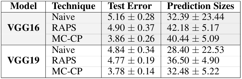
The table shows the test error and the average prediction set sizes for naive conformal prediction, RAPS conformal prediction, and MC-CP on the Tiny ImageNet dataset for two large deep learning models (a mouthful I know). It is evident that MC-CP successfully reduces the average prediction set size whilst, as a bonus, increases accuracy.

Conclusion

#

In this paper we successfully reduced overestimation in conformal prediction using our new method MC-CP. Our future work would look into enhancing MC-CP for other tasks such as object detection and image segmentation, and encoding risk-related aspects into its analysis. I encourage you to read the full paper, publish at AAAI ‘24, and check out the codebase in the GitHub repo below.

References

#

[1] Vovk, V., Gammerman, A. and Shafer, G., 2005. Algorithmic learning in a random world (Vol. 29). New York: Springer.

[2] Fan, J., Ge, J. and Mukherjee, D., 2023. UTOPIA: Universally Trainable Optimal Prediction Intervals Aggregation. arXiv preprint arXiv:2306.16549.

[3] Gal, Y. and Ghahramani, Z., 2016, June. Dropout as a bayesian approximation: Representing model uncertainty in deep learning. In international conference on machine learning (pp. 1050-1059). PMLR.

[4] Dekking, F.M., 2005. A Modern Introduction to Probability and Statistics: Understanding why and how. Springer Science & Business Media.

Codebase

#